Page 203 - Applied Statistics Using SPSS, STATISTICA, MATLAB and R

184 5 Non-Parametric Tests of Hypotheses

Note that when applying the Kolmogorov-Smirnov test, one often uses the
distribution parameters computed from the actual data. For instance, in the case of
assessing the normality of an empirical distribution, one often uses the sample
mean and sample standard deviation. This is a source of uncertainty in the
interpretation of the results.

Example 5.8
Q: Redo the previous Example 5.7 (assessing the normality of ART for class 1 of
the cork-stopper data), using the Kolmogorov-Smirnov test.
A: Running the test with SPSS we obtain the results displayed in Table 5.8,
showing no evidence (p = 0.8) supporting the rejection of the null hypothesis
(normal distribution). In R the test would be run as:

> x <- ART[1:50]
> ks.test(x, “pnorm”, mean(x), sd(x))

The following results are obtained confirming the ones in Table 5.8:

D = 0.0922, p-value = 0.7891

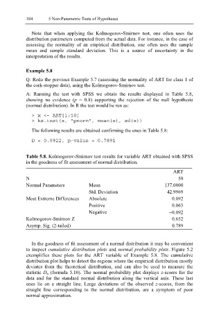
Table 5.8. Kolmogorov-Smirnov test results for variable ART obtained with SPSS
in the goodness of fit assessment of normal distribution.
ART
N 50
Normal Parameters Mean 137.0000
Std. Deviation 42.9969
Most Extreme Differences Absolute 0.092
Positive 0.063
Negative −0.092
Kolmogorov-Smirnov Z 0.652
Asymp. Sig. (2-tailed) 0.789

In the goodness of fit assessment of a normal distribution it may be convenient
to inspect cumulative distribution plots and normal probability plots. Figure 5.2
exemplifies these plots for the ART variable of Example 5.8. The cumulative
distribution plot helps to detect the regions where the empirical distribution mostly
deviates from the theoretical distribution, and can also be used to measure the
statistic D n (formula 5.10). The normal probability plot displays z-scores for the
data and for the standard normal distribution along the vertical axis. These last
ones lie on a straight line. Large deviations of the observed z-scores, from the
straight line corresponding to the normal distribution, are a symptom of poor
normal approximation.