Page 204 - Applied Statistics Using SPSS, STATISTICA, MATLAB and R

5.1 Inference on One Population 185

1
F(x) 0.99
0.9 0.98
0.8 0.95 Probability
0.90
0.7
0.75
0.6
0.5 0.50
0.4
0.25
0.3
0.10
0.2
0.05
0.1 0.02
x 0.01 Data
a 0 0 50 100 150 200 250 b 40 60 80 100 120 140 160 180 200 220 240
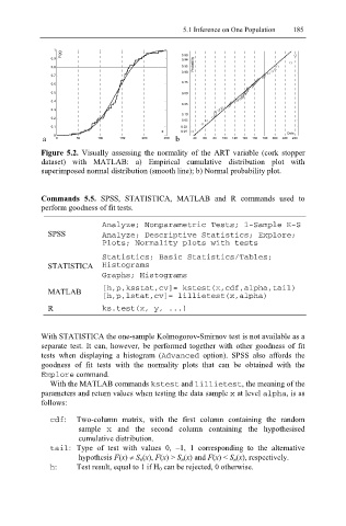
Figure 5.2. Visually assessing the normality of the ART variable (cork stopper
dataset) with MATLAB: a) Empirical cumulative distribution plot with
superimposed normal distribution (smooth line); b) Normal probability plot.

Commands 5.5. SPSS, STATISTICA, MATLAB and R commands used to
perform goodness of fit tests.

Analyze; Nonparametric Tests; 1-Sample K-S
SPSS Analyze; Descriptive Statistics; Explore;
Plots; Normality plots with tests
Statistics; Basic Statistics/Tables;
STATISTICA Histograms
Graphs; Histograms

MATLAB [h,p,ksstat,cv]= kstest(x,cdf,alpha,tail)
[h,p,lstat,cv]= lillietest(x,alpha)
R ks.test(x, y, ...)

With STATISTICA the one-sample Kolmogorov-Smirnov test is not available as a
separate test. It can, however, be performed together with other goodness of fit
tests when displaying a histogram (Advanced option). SPSS also affords the
goodness of fit tests with the normality plots that can be obtained with the
Explore command.
With the MATLAB commands kstest and lilliete st , the meaning of the
parameters and return values when testing the data sample x at level alpha , is as
follows:

cdf : Two-column matrix, with the first column containing the random
sample x and the second column containing the hypothesised
cumulative distribution.
tail : Type of test with values 0, −1, 1 corresponding to the alternative
hypothesis F(x) ≠ S n(x), F(x) > S n(x) and F(x) < S n(x), respectively.
h : Test result, equal to 1 if H 0 can be rejected, 0 otherwise.