Page 209 - Applied Statistics Using SPSS, STATISTICA, MATLAB and R

190 5 Non-Parametric Tests of Hypotheses

H 0: p 1 ≤ p 2, H 1: p 1 > p; or
H 0: p 1 ≥ p 2; H 1: p 1 < p 2.

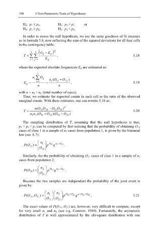
In order to assess the null hypothesis, we use the same goodness of fit measure
as in formula 5.8, now reflecting the sum of the squared deviations for all four cells
in the contingency table:

2 2 (O − E ) 2
T = ∑∑ ij ij , 5.18
= i =1 j 1 E ij

where the expected absolute frequencies E ij are estimated as:

2
n ∑ O ij
i
i
2
j
j 1
E = i 1 = = n ( O + O ) , 5.19
ij
n n

with n = n 1 + n 2 (total number of cases).
Thus, we estimate the expected counts in each cell as the ratio of the observed
marginal counts. With these estimates, one can rewrite 5.18 as:

n (O O − O O ) 2
T = 11 22 12 21 . 5.20
n 1 n 2 (O + O 21 )(O + O 22 )
11
12

The sampling distribution of T, assuming that the null hypothesis is true,
p 1 = p 2 = p, can be computed by first noticing that the probability of obtaining O 11
cases of class 1 in a sample of n 1 cases from population 1, is given by the binomial
law (see A.7):

 n 1 
P (O 11 ) =     p O 11 q n 1 O− 11 .
 O 11 

Similarly, for the probability of obtaining O 21 cases of class 1 in a sample of n 2
cases from population 2:

 n 2 
P (O 21 ) =     p O 21 q n 2 O− 21 .
 O 21 

Because the two samples are independent the probability of the joint event is
given by:

 n 1   n 2 
P (O 11 ,O 21 ) =         p O 11 O+ 21 q n− O 11 O− 21 , 5.21
 O 11   O 21 

The exact values of P(O 11, O 21) are, however, very difficult to compute, except
for very small n 1 and n 2 (see e.g. Conover, 1980). Fortunately, the asymptotic
distribution of T is well approximated by the chi-square distribution with one