Page 210 - Applied Statistics Using SPSS, STATISTICA, MATLAB and R

5.2 Contingency Tables 191

2
degree of freedom ( χ ). We then use the critical values of the chi-square
1
distribution in order to test the null hypothesis in the usual way. When dealing with
a one-sided test we face the difficulty that the T statistic does not reflect the
direction of the deviation between observed and expected frequencies. In this
situation, it is simpler to use the sampling distribution of the signed square root of
T (with the sign of O 11 O 22 − O 12 O ), which is approximated by the standard
21
normal distribution. Denoting by T 1 the signed square root of T, the one-sided test
is performed as:

H 0: p 1 ≤ p 2: reject at level α if T 1 > z 1 − α ;
H 0: p 1 ≥ p 2: reject at level α if T 1 < z α .

A “continuity correction”, known as “Yates’ correction”, is sometimes used in
the chi-square test of 2×2 contingency tables. This correction attempts to
compensate for the inaccuracy introduced by using the continuous chi-square
distribution, instead of the discrete distribution of T, as follows:

n [ O − O O | − (n ) 2 / ]| O 2
T = 11 22 12 21 . 5.22
n 1 n 2 (O + O 21 )(O + O 22 )
11
12

Example 5.9

Q: Consider the male and female populations related to the Freshmen dataset.
Based on the evidence provided by the respective samples, is it possible to
conclude that the proportion of male students that are “initiated” differs from the
proportion of female students?
A: We apply the chi-square test to the 2×2 contingency table whose rows are the
populations (variable SEX) and whose columns are the counts of initiated
freshmen (column INIT).
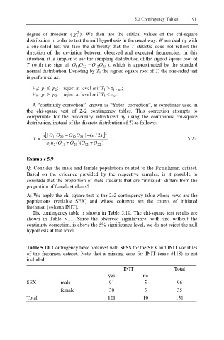
The contingency table is shown in Table 5.10. The chi-square test results are
shown in Table 5.11. Since the observed significance, with and without the
continuity correction, is above the 5% significance level, we do not reject the null
hypothesis at that level.

Table 5.10. Contingency table obtained with SPSS for the SEX and INIT variables
of the freshmen dataset. Note that a missing case for INIT (case #118) is not
included.
INIT Total
yes no
SEX male 91 5 96
female 30 5 35
Total 121 10 131