Page 208 - Applied Statistics Using SPSS, STATISTICA, MATLAB and R

5.2 Contingency Tables 189

fewer mistakes when the data was generated by asymmetric distributions, namely
the lognormal or exponential distribution. Taking into account these observations
the reader should keep in mind that the statements “a data sample can be well
modelled by the normal distribution” and a “data sample comes from a population
with a normal distribution” mean entirely different things.

5.2 Contingency Tables

Contingency tables were introduced in section 2.2.3 as a means of representing
multivariate data. In sections 2.3.5 and 2.3.6, some measures of association
computed from these tables were also presented. In this section, we describe tests
of hypotheses concerning these tables.

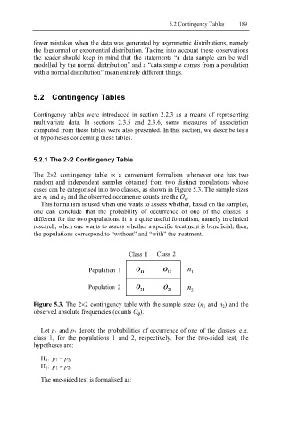
5.2.1 The 2×2 Contingency Table

The 2×2 contingency table is a convenient formalism whenever one has two
random and independent samples obtained from two distinct populations whose
cases can be categorised into two classes, as shown in Figure 5.3. The sample sizes
are n 1 and n 2 and the observed occurrence counts are the O ij.
This formalism is used when one wants to assess whether, based on the samples,
one can conclude that the probability of occurrence of one of the classes is
different for the two populations. It is a quite useful formalism, namely in clinical
research, when one wants to assess whether a specific treatment is beneficial; then,
the populations correspond to “without” and “with” the treatment.

Class 1 Class 2

Population 1 O 11 O 12 n 1

Population 2 O 21 O 22 n 2

Figure 5.3. The 2×2 contingency table with the sample sizes (n 1 and n 2) and the
observed absolute frequencies (counts O ij).

Let p 1 and p 2 denote the probabilities of occurrence of one of the classes, e.g.
class 1, for the populations 1 and 2, respectively. For the two-sided test, the
hypotheses are:

H 0: p 1 = p 2;
H 1: p 1 ≠ p 2.

The one-sided test is formalised as: