Page 213 - Applied Statistics Using SPSS, STATISTICA, MATLAB and R

194 5 Non-Parametric Tests of Hypotheses

The r×c contingency table is shown in Figure 5.4. All samples from the r
populations are assumed to be independent and randomly drawn. All observations
are assumedly categorised into exactly one of c categories. The total number of
cases is:

n = n 1 + n 2 + ...+ n r = c 1 + c 2 + ... + c c ,

where the c j are the column counts, i.e., the total number of observations in the jth
class:

r
c j = ∑ O .
ij
= i 1
Let p ij denote the probability that a randomly selected case of population i is
from class j. The hypotheses formalised for the r×c contingency table are a
generalisation of the two-sided hypotheses for the 2×2 contingency table (see
5.2.1):

H 0: For any class, the probabilities are the same for all populations: p 1j = p 2j =
… = p rj, ∀j.
H 1: There are at least two populations with different probabilities in one class:
∃ i, j, p ij ≠ p kj.

The test statistic is also a generalisation of 5.18:

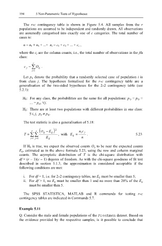
r c (O − E ) 2 n c
T = ∑∑ ij ij , with E = i j . 5.23
ij
= i 1 = j 1 E ij n

If H 0 is true, we expect the observed counts O ij to be near the expected counts
E ij, estimated as in the above formula 5.23, using the row and column marginal
counts. The asymptotic distribution of T is the chi-square distribution with
df = (r − 1)(c – 1) degrees of freedom. As with the chi-square goodness of fit test
described in section 5.1.3, the approximation is considered acceptable if the
following conditions are met:

i. For df = 1, i.e. for 2×2 contingency tables, no E ij must be smaller than 5;
ii. For df > 1, no E ij must be smaller than 1 and no more than 20% of the E ij
must be smaller than 5.

The SPSS STATISTICA, MATLAB and R commands for testing r×c
contingency tables are indicated in Commands 5.7.

Example 5.11
Q: Consider the male and female populations of the Fre shmen dataset. Based on
the evidence provided by the respective samples, is it possible to conclude that