Page 211 - Applied Statistics Using SPSS, STATISTICA, MATLAB and R

192 5 Non-Parametric Tests of Hypotheses

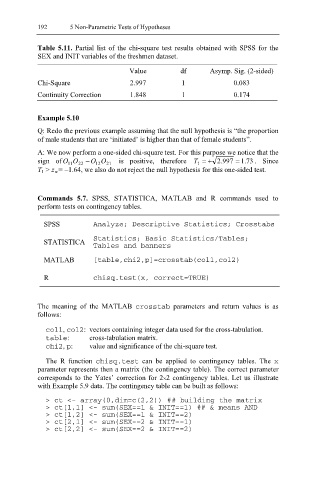
Table 5.11. Partial list of the chi-square test results obtained with SPSS for the
SEX and INIT variables of the freshmen dataset.

Value df Asymp. Sig. (2-sided)
Chi-Square 2.997 1 0.083
Continuity Correction 1.848 1 0.174

Example 5.10
Q: Redo the previous example assuming that the null hypothesis is “the proportion
of male students that are ‘initiated’ is higher than that of female students”.
A: We now perform a one-sided chi-square test. For this purpose we notice that the
sign ofO 11 O 22 − O 12 O is positive, therefore T 1 = + . 2 997 = . 1 73 . Since
21
T 1 > z α = −1.64, we also do not reject the null hypothesis for this one-sided test.

Commands 5.7. SPSS, STATISTICA, MATLAB and R commands used to
perform tests on contingency tables.

SPSS Analyze; Descriptive Statistics; Crosstabs

STATISTICA Statistics; Basic Statistics/Tables;
Tables and banners
MATLAB [table,chi2,p]=crosstab(col1,col2)

R chisq.test(x, correct=TRUE)

The meaning of the MATLAB crosstab parameters and return values is as
follows:

col1 , col2 : vectors containing integer data used for the cross-tabulation.
table : cross-tabulation matrix.
chi2 , p : value and significance of the chi-square test.

The R function chisq.te st can be applied to contingency tables. The x
parameter represents then a matrix (the contingency table). The correct parameter
corresponds to the Yates’ correction for 2×2 contingency tables. Let us illustrate
with Example 5.9 data. The contingency table can be built as follows:

> ct <- array(0,dim=c(2,2)) ## building the matrix
> ct[1,1] <- sum(SEX==1 & INIT==1) ## & means AND
> ct[1,2] <- sum(SEX==1 & INIT==2)
> ct[2,1] <- sum(SEX==2 & INIT==1)
> ct[2,2] <- sum(SEX==2 & INIT==2)