Page 216 - Applied Statistics Using SPSS, STATISTICA, MATLAB and R

5.2 Contingency Tables 197

first categorise the SCORE variable into four categories. These can be classified
as: “Poor” corresponding to a final examination score below 10; “Fair”
corresponding to a score between 10 and 13; “Good” corresponding to a score
between 14 and 16; “Very Good” corresponding to a score above 16. Let us call
PERF (performance) this new categorised variable.
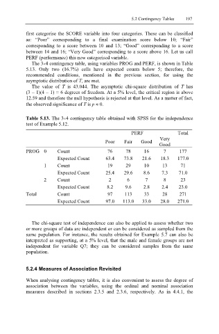
The 3×4 contingency table, using variables PROG and PERF, is shown in Table
5.13. Only two (16.7%) cells have expected counts below 5; therefore, the
recommended conditions, mentioned in the previous section, for using the
asymptotic distribution of T, are met.
The value of T is 43.044. The asymptotic chi-square distribution of T has
(3 – 1)(4 – 1) = 6 degrees of freedom. At a 5% level, the critical region is above
12.59 and therefore the null hypothesis is rejected at that level. As a matter of fact,
the observed significance of T is p ≈ 0.

Table 5.13. The 3×4 contingency table obtained with SPSS for the independence
test of Example 5.12.
PERF Total
Very
Poor Fair Good
Good
PROG 0 Count 76 78 16 7 177
Expected Count 63.4 73.8 21.6 18.3 177.0
1 Count 19 29 10 13 71
Expected Count 25.4 29.6 8.6 7.3 71.0
2 Count 2 6 7 8 23
Expected Count 8.2 9.6 2.8 2.4 23.0
Total Count 97 113 33 28 271
Expected Count 97.0 113.0 33.0 28.0 271.0

The chi-square test of independence can also be applied to assess whether two
or more groups of data are independent or can be considered as sampled from the
same population. For instance, the results obtained for Example 5.7 can also be
interpreted as supporting, at a 5% level, that the male and female groups are not
independent for variable Q7; they can be considered samples from the same
population.

5.2.4 Measures of Association Revisited

When analysing contingency tables, it is also convenient to assess the degree of
association between the variables, using the ordinal and nominal association
measures described in sections 2.3.5 and 2.3.6, respectively. As in 4.4.1, the