Page 212 - Applied Statistics Using SPSS, STATISTICA, MATLAB and R

5.2 Contingency Tables 193

An alternative and easier way to build the contingency table is by using the table
function mentioned in Commands 2.1:

> ct <- table(SEX,INIT,exclude=c(9))

Note the e xclude=c(9) argument which excludes non-valid data
(corresponding to missing data) coded with 9. Finally, we apply:

> chisq.test(ct,correct=FALSE)
X-squared = 2.9323, df = 1, p-value = 0.08682

These values agree quite well with those published in Table 5.11.
In order to solve the Example 5.12 we first recode Q7 by merging the values 1
and 2 as follows:

> Q7_12<-as.numeric(Q7<=2)+as.numeric(Q7>2)*Q7

This creates a new vector with only 4 categorical values: 1, 3, 4 and 5. The
as.numeric function converts FALSE and TRUE into 0 and 1, respectively. We
then proceed as above:

> ct<-table(SEX,Q7_12,exclude=c(9))
> chisq.test(ct)
X-squared = 5.3334, df = 3, p-value = 0.1490

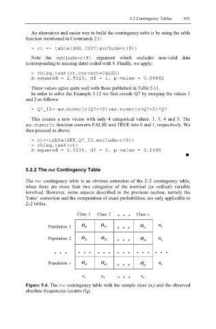
5.2.2 The rxc Contingency Table

The r×c contingency table is an obvious extension of the 2×2 contingency table,
when there are more than two categories of the nominal (or ordinal) variable
involved. However, some aspects described in the previous section, namely the
Yates’ correction and the computation of exact probabilities, are only applicable to
2×2 tables.

Class 1 Class 2 . . . Class c

Population 1 O 11 O 12 . . . O 1c n 1

Population 2 O 21 O 22 . . . O 2c n 2
. . . . . . . . . . . . . . . . . .

Population r O r1 O r2 . . . O rc n r

c 1 c 2 . . . c c
Figure 5.4. The r×c contingency table with the sample sizes (n i) and the observed
absolute frequencies (counts O ij).