Page 199 - Applied Statistics Using SPSS, STATISTICA, MATLAB and R

180 5 Non-Parametric Tests of Hypotheses

which, according to formula 5.6, has approximately a chi-square distribution with
df = k – 1 degrees of freedom. The approximation is considered acceptable if the
following conditions are met:

i. For df = 1, no E i must be smaller than 5;
ii. For df > 1, no E i must be smaller than 1 and no more than 20% of the E i
must be smaller than 5.

Expected absolute frequencies can sometimes be increased, in order to meet the
above conditions, by merging adjacent categories.
When the difference between observed (O i) and expected counts (E i) is large,
*2
the value of χ will also be large and the respective tail probability small. For a
0.95 confidence level, the critical region is above χ 2 k . 0 , 1 − 95 .

Example 5.5
Q: A die was thrown 40 times with the observed number of occurrences 8, 6, 3, 10,
7, 6, respectively for the face value running from 1 through 6. Does this sample
provide evidence that the die is not honest?
A: Table 5.5 shows the chi-square test results obtained with SPSS. Based on the
high value of the observed significance, we do not reject the null hypothesis that
the die is honest. Applying the R function c hisq.test(c(8,6,3,10,7,6))
one obtains the same results as in Table 5.5b. This function can have a second
argument with a vector of expected probabilities, which when omitted, as we did,
assigns equal probability to all categories.

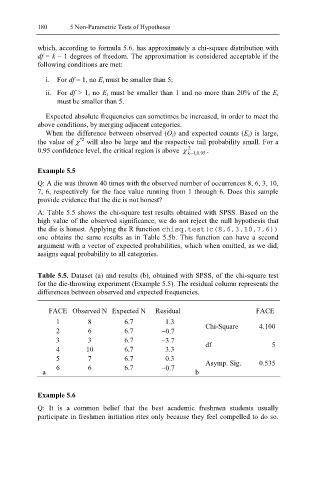
Table 5.5. Dataset (a) and results (b), obtained with SPSS, of the chi-square test
for the die-throwing experiment (Example 5.5). The residual column represents the
differences between observed and expected frequencies.

FACE Observed N Expected N Residual FACE
1 8 6.7 1.3 Chi-Square 4.100
2 6 6.7 −0.7
3 3 6.7 −3.7
4 10 6.7 3.3 df 5
5 7 6.7 0.3 0.535
6 6 6.7 −0.7 Asymp. Sig.
a b

Example 5.6
Q: It is a common belief that the best academic freshmen students usually
participate in freshmen initiation rites only because they feel compelled to do so.