Page 198 - Applied Statistics Using SPSS, STATISTICA, MATLAB and R
P. 198
5.1 Inference on One Population 179
5.1.3 The Chi-Square Goodness of Fit Test
The previous binomial test applied to a dichotomised population. When there are
more than two categories, one often wishes to assess whether the observed
frequencies of occurrence in each category are in accordance to what should be
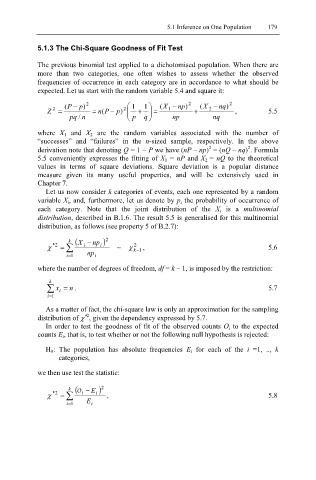
expected. Let us start with the random variable 5.4 and square it:
P ( − p) 2 2 1 1 ( X − np) 2 ( X − nq) 2
Z = = n( P − p) + = 1 + 2 , 5.5
2
pq n / p q np nq
where X 1 and X 2 are the random variables associated with the number of
“successes” and “failures” in the n-sized sample, respectively. In the above
2
2
derivation note that denoting Q = 1 − P we have (nP – np) = (nQ – nq) . Formula
5.5 conveniently expresses the fitting of X 1 = nP and X 2 = nQ to the theoretical
values in terms of square deviations. Square deviation is a popular distance
measure given its many useful properties, and will be extensively used in
Chapter 7.
Let us now consider k categories of events, each one represented by a random
variable X i, and, furthermore, let us denote by p i the probability of occurrence of
each category. Note that the joint distribution of the X i is a multinomial
distribution, described in B.1.6. The result 5.5 is generalised for this multinomial
distribution, as follows (see property 5 of B.2.7):
k (X − np ) 2
χ * 2 = ∑ i i ~ χ 2 k 1 − , 5.6
1 = i np i
where the number of degrees of freedom, df = k – 1, is imposed by the restriction:
k
∑ x = n . 5.7
i
i=1
As a matter of fact, the chi-square law is only an approximation for the sampling
∗2
distribution of χ , given the dependency expressed by 5.7.
In order to test the goodness of fit of the observed counts O i to the expected
counts E i, that is, to test whether or not the following null hypothesis is rejected:
H 0: The population has absolute frequencies E i for each of the i =1, .., k
categories,
we then use test the statistic:
k (O − E ) 2
χ * 2 = ∑ i i , 5.8
= i 1 E i

