Page 147 - Cam Design Handbook

THB5 8/15/03 1:52 PM Page 135

CAM MOTION SYNTHESIS USING SPLINE FUNCTIONS 135

10
[w] : [T] 1 [w] : [T] 2
1
1
[w] : [T] 1 [w] : [T] 2
2
2

Acceleration 0

–10
0 .5 1
Normalized time
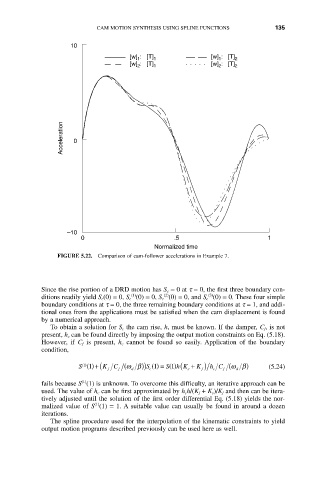
FIGURE 5.22. Comparison of cam-follower accelerations in Example 7.

Since the rise portion of a DRD motion has S c = 0 at t = 0, the first three boundary con-
(2)
(1)
(3)
ditions readily yield S c(0) = 0, S c (0) = 0, S c (0) = 0, and S c (0) = 0. These four simple
boundary conditions at t = 0, the three remaining boundary conditions at t = 1, and addi-
tional ones from the applications must be satisfied when the cam displacement is found
by a numerical approach.
To obtain a solution for S c the cam rise, h, must be known. If the damper, C f, is not
present, h c can be found directly by imposing the output motion constraints on Eq. (5.18).
However, if C f is present, h c cannot be found so easily. Application of the boundary
condition,
S 1 ()+( K C (wb )) S 1 () = () ( K ) h C (wb ) (5.24)
1 ()
h K +
S 1
f f d c s f c f d
(1)
fails because S (1) is unknown. To overcome this difficulty, an iterative approach can be
used. The value of h c can be first approximated by h c h/(K f + K s )/K f and then can be itera-
tively adjusted until the solution of the first order differential Eq. (5.18) yields the nor-
(1)
malized value of S (1) = 1. A suitable value can usually be found in around a dozen
iterations.
The spline procedure used for the interpolation of the kinematic constraints to yield
output motion programs described previously can be used here as well.