Page 153 - Cam Design Handbook

THB5 8/15/03 1:52 PM Page 141

CAM MOTION SYNTHESIS USING SPLINE FUNCTIONS 141

3
Spline (k = 10)
Optimized Polydyne

Velocity of output motion 1.5

0
0 .5 1
Normalized time
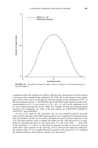
FIGURE 5.25. Normalized velocities of output motions for spline (k = 10) and optimized poly-
dyne in Example 8.

a uniform mesh for the elements are arbitrary. Based on the equal division, the first element
is located on the normalized time subdomain [0, 1/16], the second element on the subdo-
main [1/16, 2/16], and so on through the sixteenth element on the subdomain [15/16, 1].
The four Gaussian points x =±0.33992104 and ±0.86113631 of the fourth Legendre poly-
nomial defined on [-1, 1] are scaled to t = ((b - a)x + b + a)/2 on the subdomain [a, b]
for each element (Stroud and Secrest, 1986). For example, the first four Gaussian points
located on the subdomain, [0, 1/16], of the first element are 0.00433949, 0.02062747,
0.04187253, and 0.05816051.
For Eq. (5.31), there are 66 constraints—the two end conditions and the sixty-four
values for the right sides of the differential equations to be satisfied at the Gaussian points.
Sixty-six B-splines of order six are used to formulate the system of linear equations in Eq.
(5.6). The knot sequence used to evaluate the splines for the collocation process is estab-
lished by repeating four knots at each mesh point, t = 1/16, 2/16, 3/16,... , and 15/16.
At the end points, t = 0 and t = 1, the knots are repeated six times as necessary because
of the order of the spliones (k = 6). After Eq. (5.6) is solved for the unknown coefficients,
the solution of Eq. (5.31) is readily found for any point in the interval 0 £ t £ 1 enabling
the dynamic behavior of the follower system to be determined.