Page 154 - Cam Design Handbook

THB5 8/15/03 1:53 PM Page 142

142 CAM DESIGN HANDBOOK

10

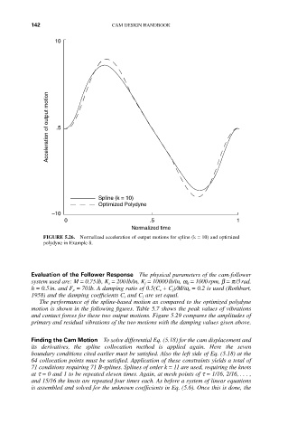
Acceleration of output motion .5

Spline (k = 10)
Optimized Polydyne
–10
0 .5 1
Normalized time
FIGURE 5.26. Normalized acceleration of output motions for spline (k = 10) and optimized
polydyne in Example 8.

Evaluation of the Follower Response The physical parameters of the cam-follower
system used are: M = 0.75lb, K s = 200lb/in, K f = 10000lb/in, w d = 1000rpm, b = p/3rad.
h = 0.5in. and F p = 70lb. A damping ratio of 0.5(C s + C f)/M/w n = 0.2 is used (Rothbart,
1958) and the damping coefficients C s and C f are set equal.
The performance of the spline-based motion as compared to the optimized polydyne
motion is shown in the following figures. Table 5.7 shows the peak values of vibrations
and contact forces for these two output motions. Figure 5.29 compares the amplitudes of
primary and residual vibrations of the two motions with the damping values given above.

Finding the Cam Motion To solve differential Eq. (5.18) for the cam displacement and
its derivatives, the spline collocation method is applied again. Here the seven
boundary conditions cited earlier must be satisfied. Also the left side of Eq. (5.18) at the
64 collocation points must be satisfied. Application of these constraints yields a total of
71 conditions requiring 71 B-splines. Splines of order k = 11 are used, requiring the knots
at t = 0 and 1 to be repeated eleven times. Again, at mesh points of t = 1/16, 2/16,... ,
and 15/16 the knots are repeated four times each. As before a system of linear equations
is assembled and solved for the unknown coefficients in Eq. (5.6). Once this is done, the