Page 69 - Circuit Analysis II with MATLAB Applications

Series Resonance

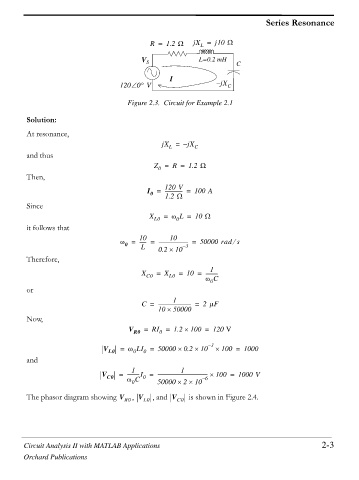
R = 1.2 : jX = j10 :
L
`
V S L=0.2 mH C

I
120 0q V j – X C
‘
Figure 2.3. Circuit for Example 2.1

Solution:
At resonance,
jX = – jX C
L
and thus
Z = R = 1.2 :
0
Then,
120 V
I = -------------- = 100 A
0
1.2 :
Since
X L0 = Z L = 10 :
0
it follows that
10 10
Z = ------ = ------------------------ = 50000 rad s
e
0
–
L
3
10
0.2 u
Therefore,
1
X C0 = X L0 = 10 = ----------
Z C
0
or
1
C = --------------------------- = 2 PF
10 u 50000
Now,
V R0 = RI = 1.2 u 100 = 120 V
0
– 3
V L0 = Z LI = 50000 u 0.2 u 10 u 100 = 1000
0
0
and
1 1
V C0 = ----------I = ----------------------------------------- u 100 = 1000 V
0
Z C
0 50000 u 2 u 10 – 6
The phasor diagram showing V R0 , V L0 , and V C0 is shown in Figure 2.4.

Circuit Analysis II with MATLAB Applications 2-3
Orchard Publications