Page 55 - Computational Retinal Image Analysis

3 Ophthalmic instruments 45

To process the signal, the processing unit PU performs an apparent simple math-
ematical operation to generate an A-scan: a Fast Fourier Transform (FFT) of the
electrical signal, proportional to the photo-detected spectrum. However, due to the
nonlinearities in the spectrometer, an irregular modulation (chirp) of the electrical
signal read out by the spectrometer occurs. An unbalanced dispersion in the interfer-
ometer and the sample itself [54] can also contribute to the chirp. Unless this chirp
is compensated for, after sophisticated linearization procedures, an FFT applied to
the electrical signal leads to a wider and at the same time, reduced amplitude of the
reflectivity profile peaks. Imperfections in these procedures become more obvious at
larger OPD values in the interferometer and more pronounced as the spectral band-
width is increased.
By collecting a succession of A-scans as the optical beam laterally scans the
sample, a cross-section image is produced (as illustrated in Fig. 20). For each lateral
position x i , A-scans are obtained with no need of any mechanical movements. Thus,
a number of P A-scans are ensembled together to produce, a B-scan CB-OCT im-
age of size P × Q. Here, Q is typically half the number of points used to digitize the
spectrum (i.e., the number of pixels in the linear camera employed).
Generating real-time A-scans in CB-OCT is quite challenging. The frequency
at which spectra are acquired is typically over 100 kHz. This mean that to ensure a
real-time operation, the FFT operation must not take longer than 10 μs. This is pos-
sible using a modern multicore PC however the electric signal must be corrected for
chirping before FFT via time consuming sequential interpolation procedures. As CB-
OCT and TD-OCT instruments are using the same optical sources, they will deliver
images with similar axial resolutions.
In terms of sensitivity, CB-OCT has a 20–30 dB advantage over TD-OCT [55],
however a limited axial imaging range due to the finite size of camera's pixels. The
production of en-face CB-OCT images is done in a manner similar to axial TD-OCT,
i.e., by rendering the en-face view from the 3D volume. The acquisition time of the

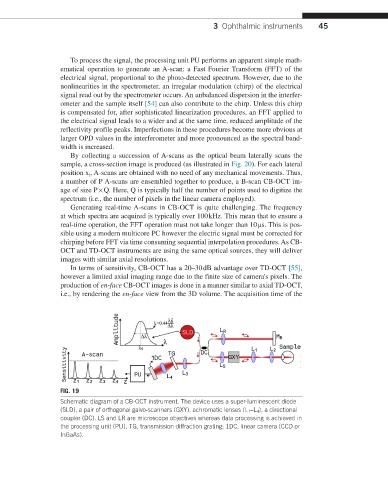
FIG. 19
Schematic diagram of a CB-OCT instrument. The device uses a super-luminescent diode
(SLD), a pair of orthogonal galvo-scanners (GXY), achromatic lenses (L 1 –L 4 ), a directional
coupler (DC). LS and LR are microscope objectives whereas data processing is achieved in
the processing unit (PU). TG, transmission diffraction grating; 1DC, linear camera (CCD or
InGaAs).