Page 176 - Computational Statistics Handbook with MATLAB

Chapter 5: Exploratory Data Analysis 163

0

1 2 3 4 5 6 7
GU
U
F F F FI II IG URE GU 5.3 RE RE RE 5.3 7 7 7 7
5.3
5.3
G
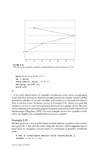
This shows the parallel coordinate representation for the 4-D point (1,3,7,2).
plot(c,0:3,c,0:3,'*')
ax = axis;
axis([ax(1) ax(2) -1 4 ])
set(gca,'ytick',0)
hold off

If we plot observations in parallel coordinates with colors designating
what class they belong to, then the parallel coordinate display can be used to
determine whether or not the variables will enable us to separate the classes.
This is similar to the Andrews curves in Example 5.23, where we used the
Andrews curves to view the separation between two species of iris. The par-
allel coordinate plot provides graphical representations of multi-dimensional
relationships [Wegman, 1990]. The next example shows how parallel coordi-
nates can display the correlation between two variables.

Example 5.25
We first generate a set of 20 bivariate normal random variables with correla-
tion given by 1. We plot the data using the function called csparallel to
show how to recognize various types of correlation in parallel coordinate
plots.

% Get a covariance matrix with correlation 1.
covmat = [1 1; 1 1];

© 2002 by Chapman & Hall/CRC