Page 175 - Computational Statistics Handbook with MATLAB

162 Computational Statistics Handbook with MATLAB

in Equation 5.9. Embrechts and Herzberg [1991] also suggest that the data be
rescaled so they are centered at the origin and have covariance equal to the
identity matrix. Andrews curves can be extended by using orthogonal bases
other than sines and cosines. For example, Embrechts and Herzberg [1991]
illustrate Andrews curves using Legendre polynomials and Chebychev poly-
nomials.

r
CooCoo
a
rdindin
Par
PPaarr aall
Pa raal ll ll leel eell l CooCoo rr dindin aatt tees eess s
at
In the Cartesian coordinate system the axes are orthogonal, so the most we
can view is three dimensions. If instead we draw the axes parallel to each
other, then we can view many axes on the same display. This technique was
developed by Wegman [1986] as a way of viewing and analyzing multi-
dimensional data and was introduced by Inselberg [1985] in the context of
computational geometry and computer vision. Parallel coordinate tech-
niques were expanded on and described in a statistical setting by Wegman
[1990]. Wegman [1990] also gave a rigorous explanation of the properties of
parallel coordinates as a projective transformation and illustrated the duality
properties between the parallel coordinate representation and the Cartesian
orthogonal coordinate representation.
A parallel coordinate plot for d-dimensional data is constructed by draw-
ing d lines parallel to each other. We draw d copies of the real line represent-
ing the coordinates for x 1 x 2 … x d ., , , The lines are the same distance apart and
are perpendicular to the Cartesian y axis. Additionally, they all have the same
positive orientation as the Cartesian x axis. Some versions of parallel coordi-
nates [Inselberg, 1985] draw the parallel axes perpendicular to the Cartesian
x axis.
,
,
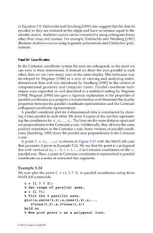
A point C = ( c 1 … c 4 ) is shown in Figure 5.37 with the MATLAB code
that generates it given in Example 5.24. We see that the point is a polygonal
,
line with vertices at c i i –,( 1) i = 1 … d in Cartesian coordinates on the x i
,
,
parallel axis. Thus, a point in Cartesian coordinates is represented in parallel
coordinates as a series of connected line segments.
Example 5.24
,,,
We now plot the point C = ( 1 372) in parallel coordinates using these
MATLAB commands.
c = [1 3 7 2];
% Get range of parallel axes.
x = [1 7];
% Plot the 4 parallel axes.
plot(x,zeros(1,2),x,ones(1,2),x,...
2*ones(1,2),x,3*ones(1,2))
hold on
% Now plot point c as a polygonal line.

© 2002 by Chapman & Hall/CRC