Page 170 - Computational Statistics Handbook with MATLAB

Chapter 5: Exploratory Data Analysis 157

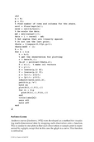
clf
n = 8;
p = 11;
% Find number of rows and columns for the stars.
ncol = floor(sqrt(n));
nrow = ceil(n/ncol);
% Re-scale the data.
md = min(cereal(:));
data = 1 + cereal - md;
% Get angles that are linearly spaced.
% Do not use the last point.
theta = linspace(0,2*pi,p+1);
theta(end) = [];
k = 0;
for i = 1:n
k = k+1;
% get the observation for plotting
r = data(k,:);
[x,y] = pol2cart(theta,r);
X = x(:); % make col vectors
Y = y(:);
X = [zeros(p,1) X];
Y = [zeros(p,1) Y];
x = [x(:); x(1)];
y = [y(:); y(1)];
subplot(nrow,ncol,k),
patch(x,y,'w')
hold on
plot(X(1,:),Y(1,:))
for ii = 2:p
plot(X(ii,:),Y(ii,:))
end
title(labs{k})
axis off
hold off
end

urve
es
C
urv
AndrewsC
Andrews CC urvurv eess s
AndrewsAndrews
Andrews curves [Andrews, 1972] were developed as a method for visualiz-
ing multi-dimensional data by mapping each observation onto a function.
This is similar to star plots in that each observation or sample point is repre-
sented by a glyph, except that in this case the glyph is a curve. This function
is defined as
© 2002 by Chapman & Hall/CRC