Page 168 - Computational Statistics Handbook with MATLAB

Chapter 5: Exploratory Data Analysis 155

FI F U URE G 5.3 RE 5.3 2 2
IG
5.3
GU
F F II GU RE RE 5.3 2 2
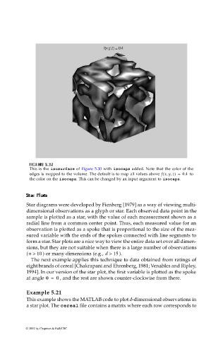
This is the isosurface of Figure 5.30 with isocaps added. Note that the color of the
edges is mapped to the volume. The default is to map all values above f xy z,,( ) = 0.4 to
the color on the isocaps. This can be changed by an input argument to isocaps.
SStata
Sta
Sta r r rr Plot PlotPlot Plots s ss
Star diagrams were developed by Fienberg [1979] as a way of viewing multi-
dimensional observations as a glyph or star. Each observed data point in the
sample is plotted as a star, with the value of each measurement shown as a
radial line from a common center point. Thus, each measured value for an
observation is plotted as a spoke that is proportional to the size of the mea-
sured variable with the ends of the spokes connected with line segments to
form a star. Star plots are a nice way to view the entire data set over all dimen-
sions, but they are not suitable when there is a large number of observations
(n > 10 ) or many dimensions (e.g., d > 15 ).
The next example applies this technique to data obtained from ratings of
eight brands of cereal [Chakrapani and Ehrenberg, 1981; Venables and Ripley,
1994]. In our version of the star plot, the first variable is plotted as the spoke
at angle θ = 0 , and the rest are shown counter-clockwise from there.

Example 5.21
This example shows the MATLAB code to plot d-dimensional observations in
a star plot. The cereal file contains a matrix where each row corresponds to

© 2002 by Chapman & Hall/CRC