Page 164 - Computational Statistics Handbook with MATLAB

Chapter 5: Exploratory Data Analysis 151

0.06
3
0.05
2
1 0.04
Z Axis 0
−1
0.03
−2
−3
3 0.02
2
1 0.01
0 2 3
−1 0 1
−2 −1
Y Axis −2
−3 −3 X Axis

IG
,
F FI U URE G 5.2 RE 5.2 8 8
,
5.2
F F II GU RE RE 5.2 8 8
GU
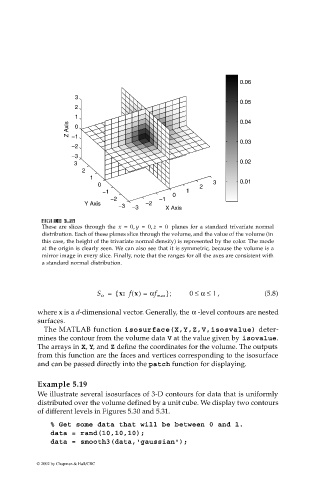
These are slices through the x = 0 y = 0 z = 0 planes for a standard trivariate normal
distribution. Each of these planes slice through the volume, and the value of the volume (in
this case, the height of the trivariate normal density) is represented by the color. The mode
at the origin is clearly seen. We can also see that it is symmetric, because the volume is a
mirror image in every slice. Finally, note that the ranges for all the axes are consistent with
a standard normal distribution.
S α = { x: f x() = αf max }; 0 ≤ α ≤ , 1 (5.8)
α
where x is a d-dimensional vector. Generally, the -level contours are nested
surfaces.
The MATLAB function isosurface(X,Y,Z,V,isosvalue) deter-
mines the contour from the volume data V at the value given by isovalue.
The arrays in X, Y, and Z define the coordinates for the volume. The outputs
from this function are the faces and vertices corresponding to the isosurface
and can be passed directly into the patch function for displaying.

Example 5.19
We illustrate several isosurfaces of 3-D contours for data that is uniformly
distributed over the volume defined by a unit cube. We display two contours
of different levels in Figures 5.30 and 5.31.
% Get some data that will be between 0 and 1.
data = rand(10,10,10);
data = smooth3(data,'gaussian');

© 2002 by Chapman & Hall/CRC