Page 165 - Computational Statistics Handbook with MATLAB

152 Computational Statistics Handbook with MATLAB

0.06
0.05
0.04
0.03
0.02
0.01

2 3
2
0 1
0
−2 −2 −1
Y Axis −3 X Axis

GU
5.2
F F FI F II IG URE G 5.2 RE RE RE 5.2 9 9 9 9
U
5.2
GU
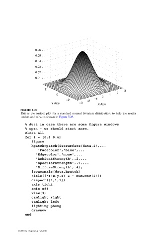
This is the surface plot for a standard normal bivariate distribution. to help the reader
understand what is shown in Figure 5.28.
% Just in case there are some figure windows
% open - we should start anew.
close all
for i = [0.4 0.6]
figure
hpatch=patch(isosurface(data,i),...
'Facecolor','blue',...
'Edgecolor','none',...
'AmbientStrength',.2,...
'SpecularStrength',.7,...
'DiffuseStrength',.4);
isonormals(data,hpatch)
title(['f(x,y,z) = ' num2str(i)])
daspect([1,1,1])
axis tight
axis off
view(3)
camlight right
camlight left
lighting phong
drawnow
end

© 2002 by Chapman & Hall/CRC