Page 166 - Computational Statistics Handbook with MATLAB

Chapter 5: Exploratory Data Analysis 153

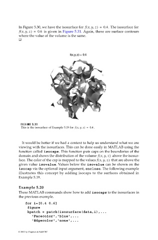
In Figure 5.30, we have the isosurface for f xy z,,( ) = 0.4. The isosurface for
(
,,
f xy z) = 0.6 is given in Figure 5.31. Again, these are surface contours
where the value of the volume is the same.

F FI U URE G 5.3 RE 5.3 0 0
,,
(
IG
F F II GU RE RE 5.3 0 0
GU
5.3
This is the isosurface of Example 5.19 for f xy z) = 0.4 .
It would be better if we had a context to help us understand what we are
viewing with the isosurfaces. This can be done easily in MATLAB using the
function called isocaps. This function puts caps on the boundaries of the
domain and shows the distribution of the volume f xy z,,( ) above the isosur-
face. The color of the cap is mapped to the values f xy z,,( ) that are above the
given value isovalue. Values below the isovalue can be shown on the
isocap via the optional input argument, enclose. The following example
illustrates this concept by adding isocaps to the surfaces obtained in
Example 5.19.

Example 5.20
These MATLAB commands show how to add isocaps to the isosurfaces in
the previous example.
for i=[0.4 0.6]
figure
hpatch = patch(isosurface(data,i),...
'Facecolor','blue',...
'Edgecolor','none',...

© 2002 by Chapman & Hall/CRC