Page 171 - Computational Statistics Handbook with MATLAB

158 Computational Statistics Handbook with MATLAB

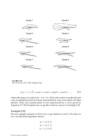
Cereal 1 Cereal 2

Cereal 3 Cereal 4

Cereal 5 Cereal 6

Cereal 7 Cereal 8

G
II
U
5.3
5.3
GU
F F FI F IG URE GU 5.3 RE RE RE 5.3 4 4 4 4
This is the star plot of the cereal data.
f x t() = x 1 ⁄ 2 + x 2 sin + x 3 cos + x 4 sin 2t + x 5 cos 2t + … , (5.9)
t
t
where the range of t is given by π– ≤≤ π . Each observation is projected onto
t
a set of orthogonal basis functions represented by sines and cosines and then
plotted. Thus, each sample point is now represented by a curve given by
Equation 5.9. We illustrate how to get the Andrews curves in Example 5.22.

Example 5.22
We use a simple example to show how to get Andrews curves. The data we
have are the following observations:

,,
x = ( 26 4)
1
,,
x 2 = ( 57 3)
,,
x 3 = ( 18 9).
© 2002 by Chapman & Hall/CRC