Page 173 - Computational Statistics Handbook with MATLAB

160 Computational Statistics Handbook with MATLAB

It has been shown [Andrews, 1972; Embrechts and Herzberg, 1991] that
because of the mathematical properties of the trigonometric functions, the
Andrews curves preserve means, distance (up to a constant) and variances.
One consequence of this is that Andrews curves showing functions close
together suggest that the corresponding data points will also be close
together. Thus, one use of Andrews curves is to look for clustering of the data
points.

Example 5.23
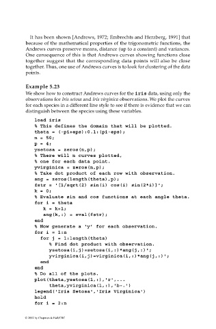
We show how to construct Andrews curves for the iris data, using only the
observations for Iris setosa and Iris virginica observations. We plot the curves
for each species in a different line style to see if there is evidence that we can
distinguish between the species using these variables.
load iris
% This defines the domain that will be plotted.
theta = (-pi+eps):0.1:(pi-eps);
n = 50;
p = 4;
ysetosa = zeros(n,p);
% There will n curves plotted,
% one for each data point.
yvirginica = zeros(n,p);
% Take dot product of each row with observation.
ang = zeros(length(theta),p);
fstr = '[1/sqrt(2) sin(i) cos(i) sin(2*i)]';
k = 0;
% Evaluate sin and cos functions at each angle theta.
for i = theta
k = k+1;
ang(k,:) = eval(fstr);
end
% Now generate a ‘y’ for each observation.
for i = 1:n
for j = 1:length(theta)
% Find dot product with observation.
ysetosa(i,j)=setosa(i,:)*ang(j,:)';
yvirginica(i,j)=virginica(i,:)*ang(j,:)';
end
end
% Do all of the plots.
plot(theta,ysetosa(1,:),'r',...
theta,yvirginica(1,:),'b-.')
legend('Iris Setosa','Iris Virginica')
hold
for i = 2:n

© 2002 by Chapman & Hall/CRC