Page 174 - Computational Statistics Handbook with MATLAB

Chapter 5: Exploratory Data Analysis 161

plot(theta,ysetosa(i,:),'r',...
theta,yvirginica(i,:),'b-.')
end
hold off
title('Andrews Plot')
xlabel('t')
ylabel('Andrews Curve')
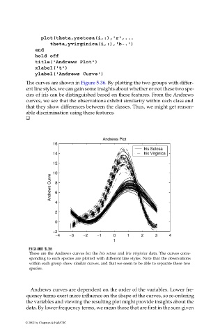
The curves are shown in Figure 5.36. By plotting the two groups with differ-
ent line styles, we can gain some insights about whether or not these two spe-
cies of iris can be distinguished based on these features. From the Andrews
curves, we see that the observations exhibit similarity within each class and
that they show differences between the classes. Thus, we might get reason-
able discrimination using these features.

Andrews Plot
16
Iris Setosa
14 Iris Virginica
12

10
Andrews Curve 8

6
4
2

0
−2
−4 −3 −2 −1 0 1 2 3 4
t
IG
F FI U URE G 5.3 RE 5.3 6 6
GU
F F II GU RE RE 5.3 6 6
5.3
These are the Andrews curves for the Iris setosa and Iris virginica data. The curves corre-
sponding to each species are plotted with different line styles. Note that the observations
within each group show similar curves, and that we seem to be able to separate these two
species.
Andrews curves are dependent on the order of the variables. Lower fre-
quency terms exert more influence on the shape of the curves, so re-ordering
the variables and viewing the resulting plot might provide insights about the
data. By lower frequency terms, we mean those that are first in the sum given

© 2002 by Chapman & Hall/CRC