Page 172 - Computational Statistics Handbook with MATLAB

Chapter 5: Exploratory Data Analysis 159

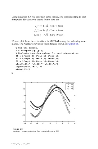
Using Equation 5.9, we construct three curves, one corresponding to each
data point. The Andrews curves for the data are:

f x t() = 2 ⁄ 2 + 6sin + 4 cos t
t
1
t
f x t() = 5 ⁄ 2 + 7sin + 3 cos t
2
t
f x t() = 1 ⁄ 2 + 8sin + 9cos t.
3
We can plot these three functions in MATLAB using the following com-
mands. The Andrews curves for these data are shown in Figure 5.35.
% Get the domain.
t = linspace(-pi,pi);
% Evaluate function values for each observation.
f1 = 2/sqrt(2)+6*sin(t)+4*cos(t);
f2 = 5/sqrt(2)+7*sin(t)+3*cos(t);
f3 = 1/sqrt(2)+8*sin(t)+9*cos(t);
plot(t,f1,'.',t,f2,'*',t,f3,'o')
legend('F1','F2','F3')
xlabel('t')

15
F1
F2
10 F3

5

0

−5

−10

−15
−4 −3 −2 −1 0 1 2 3 4
t

GU
IG
F FI F F II U URE G 5.3 RE RE RE 5.3 5 5 5 5
5.3
5.3
GU
Andrews curves for the three data points in Example 5.22.
© 2002 by Chapman & Hall/CRC