Page 163 - Computational Statistics Handbook with MATLAB

150 Computational Statistics Handbook with MATLAB

Virginica
8
6 Sepal Length
4
4

3 Sepal Width
2
8
6 Petal Length
4
3
2 Petal Width
1
4 6 8 2 3 4 4 6 8 1 2 3

GU
5.2
5.2
U
FI F F F II IG URE G 5.2 RE RE RE 5.2 7 7 7 7
GU
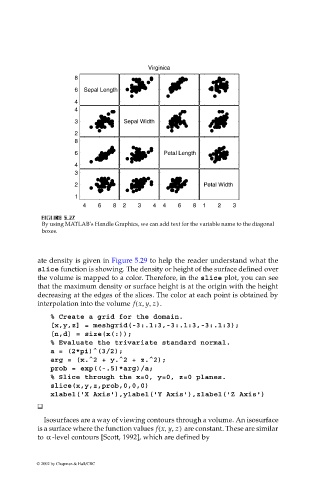
By using MATLAB’s Handle Graphics, we can add text for the variable name to the diagonal
boxes.
ate density is given in Figure 5.29 to help the reader understand what the
slice function is showing. The density or height of the surface defined over
the volume is mapped to a color. Therefore, in the slice plot, you can see
that the maximum density or surface height is at the origin with the height
decreasing at the edges of the slices. The color at each point is obtained by
interpolation into the volume f xy z,,( ) .

% Create a grid for the domain.
[x,y,z] = meshgrid(-3:.1:3,-3:.1:3,-3:.1:3);
[n,d] = size(x(:));
% Evaluate the trivariate standard normal.
a = (2*pi)^(3/2);
arg = (x.^2 + y.^2 + z.^2);
prob = exp((-.5)*arg)/a;
% Slice through the x=0, y=0, z=0 planes.
slice(x,y,z,prob,0,0,0)
xlabel('X Axis'),ylabel('Y Axis'),zlabel('Z Axis')

Isosurfaces are a way of viewing contours through a volume. An isosurface
is a surface where the function values f xy z,,( ) are constant. These are similar
α
to -level contours [Scott, 1992], which are defined by

© 2002 by Chapman & Hall/CRC