Page 281 - DSP Integrated Circuits

266 Chapter 6 DSP Algorithms

6.9.3 Scattered Look-Ahead Pipelining

In the scattered look-ahead pipelining approach, the transfer function is modified
such that the pipelined filter has poles with equal spacing around the origin [16,
18, 19, 26]. The effect of the added poles is canceled by the corresponding zeros.
M
The denominator will contain only powers of Z where M is the number of pipeline
stages. The filter output is therefore computed from past values that are scattered
in time, i.e., y(n - M), y(n - 2M), y(n - 3M),... ,y(n - NM) where N is the order of
the original filter. In fact, this technique is the same as the state-decimation tech-
nique discussed in section 6.9.1. This approach always leads to stable filters. We
illustrate the scattered look-ahead pipelining technique by a few examples.

EXAMPLE 6.13
Apply scattered look-ahead pipelining to a first-order filter. The pipeline shall have
four stages.
The original filter is described by the transfer function

which corresponds to the difference equation

We add M - 1 poles and zeros at z = b eJ 2nk/M for k = 1, 2,..., M - 1. The
transfer function becomes

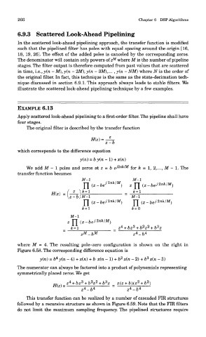
where M = 4. The resulting pole-zero configuration is shown on the right in
Figure 6.58. The corresponding difference equation is

The numerator can always be factored into a product of polynomials representing
symmetrically placed zeros. We get

This transfer function can be realized by a number of cascaded FIR structures
followed by a recursive structure as shown in Figure 6.59. Note that the FIR filters
do not limit the maximum sampling frequency. The pipelined structures require