Page 303 - Decision Making Applications in Modern Power Systems

Particle swarm optimization applied Chapter | 10 263

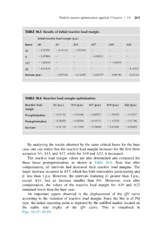
TABLE 10.5 Results of initial reactive load margin.
Initial reactive load margin (p.u.)
Buses A0 A1 A11 A17 A19 A22
41 2 4.35951 2 4.43132 2 4.52346

9 2 5.97804 2 6.00551
117 2 1.48549 2 1.40359
29 2 4.67670 2 4.41537
Increase (p.u.) 2 0.07181 2 0.16395 2 0.02747 0.08190 0.26133

TABLE 10.6 Reactive load margin-optimization.

Reactive load A1 (p.u.) A11 (p.u.) A17 (p.u.) A19 (p.u.) A22 (p.u.)
margin
Preoptimization 2 4.43132 2 4.52346 2 6.00551 2 1.40359 2 4.41537
Postoptimization 2 4.58260 2 4.64384 2 6.19161 2 1.43564 2 4.47146
Increase 2 0.15128 2 0.12038 2 0.18609 2 0.03206 2 0.05609

By analyzing the results obtained by the same critical buses for the base
case, one can notice that the reactive load margin increases for the first three
scenarios A1, A11, and A17, while for A19 and A22, it decreased.
The reactive load margin values are also determined and compared for
these buses postoptimization, as shown in Table 10.6. Note that after
compensation, all intervals had increased their reactive load margins. The
larger increase occurred in A17, which has both renewables participating and
fc less than 1 p.u. However, the intervals featuring fc greater than 1 p.u.,
except A11, had an increase smaller than 6%. Moreover, even after
compensation, the values of the reactive load margin for A19 and A22
remained lower than the base case.
An important aspect observed is the displacement of the QV curve
according to the variation of reactive load margin. Since the bus is of PQ
type, the initial operating point is depicted by the unfilled marker located on
the stable side (right) of the QV curve. This is visualized in
Figs. 10.15 10.19.