Page 505 - Design for Six Sigma a Roadmap for Product Development

464 Chapter Twelve

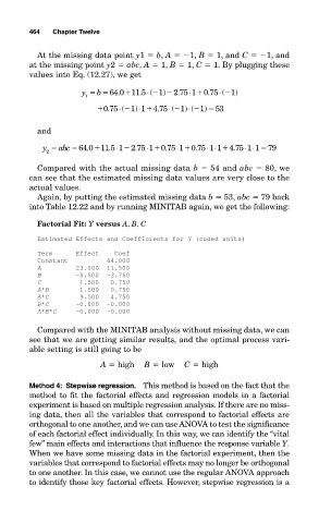
At the missing data point y1 b, A 1, B 1, and C 1, and
at the missing point y2 abc, A 1, B 1, C 1. By plugging these
values into Eq. (12.27), we get
⋅
⋅
⋅
y 64 0 11 5 2 75 1 0 75 1)

(
1
)
b
.
.
(
.
.
1
⋅
⋅
1
0 .75⋅ ( 1 1 4 .75⋅ ( 1 ) ( 53
)
)
and
⋅
⋅
⋅
⋅⋅
⋅
⋅

y abc 64 0 11 5 1 2 75 1 0 75 1 0 75 1 1 4..75 1 1 79

.
.
.
.
.
2
Compared with the actual missing data b 54 and abc 80, we
can see that the estimated missing data values are very close to the
actual values.
Again, by putting the estimated missing data b 53, abc 79 back
into Table 12.22 and by running MINITAB again, we get the following:
Factorial Fit: Y versus A, B, C
Estimated Effects and Coefficients for Y (coded units)
Term Effect Coef
Constant 64.000
A 23.000 11.500
B -5.500 -2.750
C 1.500 0.750
A*B 1.500 0.750
A*C 9.500 4.750
B*C -0.000 -0.000
A*B*C -0.000 -0.000
Compared with the MINITAB analysis without missing data, we can
see that we are getting similar results, and the optimal process vari-
able setting is still going to be
A high B low C high
Method 4: Stepwise regression. This method is based on the fact that the
method to fit the factorial effects and regression models in a factorial
experiment is based on multiple regression analysis. If there are no miss-
ing data, then all the variables that correspond to factorial effects are
orthogonal to one another, and we can use ANOVA to test the significance
of each factorial effect individually. In this way, we can identify the “vital
few” main effects and interactions that influence the response variable Y.
When we have some missing data in the factorial experiment, then the
variables that correspond to factorial effects may no longer be orthogonal
to one another. In this case, we cannot use the regular ANOVA approach
to identify those key factorial effects. However, stepwise regression is a