Page 500 - Design for Six Sigma a Roadmap for Product Development

Fundamentals of Experimental Design 459

Each interaction can also be decomposed into several elementary
interaction effects. For example, in Eq. (12.18), we can identify the fol-
lowing two elementary interaction effects:
ab a b 1: effect of AB when C is at low level
abc ac bc c: effect of A when C is at high level

From Eq. (12.18) we can get
1 ⎡
AB 1−− − − abc ⎦ ⎤
4 ⎣
ab ab c acbc
⎡ (ab a b (abc ac bc ) ⎤ ⎦ (12.23)
−−
−
−
2 2 ⎣
1
1
c
)
1 1
2
Equation (12.23) clearly indicates that AB is the average of two
elementary interaction effects; we can derive the similar equations to
Eq. (12.23) for other two-factor interaction effects. In general, for a 2 k
factorial experiment, each two-factor interaction effect is the arith-
metic average of its 2 k 2 elementary interaction effects.
After we showed the fact that each factorial effect is the arithmetic
average of several elementary effects, when we have a few missing
runs in factorial experiments, it may affect only a small number of ele-
mentary effects; so the main effects or interactions can still be esti-
mated by the partial average of the remaining elementary effects. We
will show this method in Example 12.10.
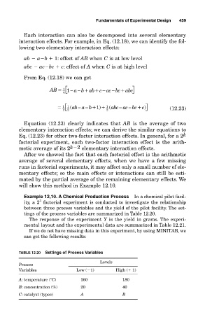
Example 12,10. A Chemical Production Process In a chemical pilot facil-
3
ity, a 2 factorial experiment is conducted to investigate the relationship
between three process variables and the yield of the pilot facility. The set-
tings of the process variables are summarized in Table 12.20.
The response of the experiment Y is the yield in grams. The experi-
mental layout and the experimental data are summarized in Table 12.21.
If we do not have missing data in this experiment, by using MINITAB, we
can get the following results:

TABLE 12.20 Settings of Process Variables

Levels
Process
Variables Low ( 1) High ( 1)
A: temperature ( C) 160 180
B: concentration (%) 20 40
C: catalyst (types) A B