Page 499 - Design for Six Sigma a Roadmap for Product Development

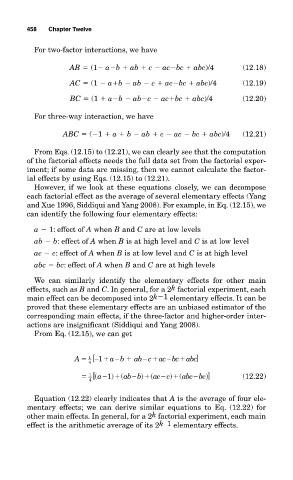
458 Chapter Twelve

For two-factor interactions, we have

AB (1 a b ab c ac bc abc)/4 (12.18)
AC (1 a b ab c ac bc abc)/4 (12.19)

BC (1 a b ab c ac bc abc)/4 (12.20)

For three-way interaction, we have

ABC ( 1 a b ab c ac bc abc)/4 (12.21)

From Eqs. (12.15) to (12.21), we can clearly see that the computation
of the factorial effects needs the full data set from the factorial exper-
iment; if some data are missing, then we cannot calculate the factor-
ial effects by using Eqs. (12.15) to (12.21).
However, if we look at these equations closely, we can decompose
each factorial effect as the average of several elementary effects (Yang
and Xue 1996, Siddiqui and Yang 2008). For example, in Eq. (12.15), we
can identify the following four elementary effects:

a 1: effect of A when B and C are at low levels
ab b: effect of A when B is at high level and C is at low level
ac c: effect of A when B is at low level and C is at high level
abc bc: effect of A when B and C are at high levels

We can similarly identify the elementary effects for other main
k
effects, such as B and C. In general, for a 2 factorial experiment, each
main effect can be decomposed into 2 k 1 elementary effects. It can be
proved that these elementary effects are an unbiased estimator of the
corresponding main effects, if the three-factor and higher-order inter-
actions are insignificant (Siddiqui and Yang 2008).
From Eq. (12.15), we can get

A [ − 1 a b ab c ac bc abc]
−
−
−
1
4
[ ( a 1) ( ab b))(ac c )(abc bc )] (12.22)
−
−
−
−

1
4
Equation (12.22) clearly indicates that A is the average of four ele-
mentary effects; we can derive similar equations to Eq. (12.22) for
k
other main effects. In general, for a 2 factorial experiment, each main
effect is the arithmetic average of its 2 k 1 elementary effects.