Page 498 - Design for Six Sigma a Roadmap for Product Development

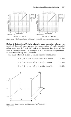
Fundamentals of Experimental Design 457

Half normal plot of the effects Half normal plot of the effects
(response is Y, Alpha = 0.05) (response is Y, Alpha = 0.05)
Effect type Effect type
98 Not significant 98 Not significant
Significant Significant
95 95
Factor Name Factor Name
A A A A
90 B B 90 B B
Percent 85 C C Percent 85 C C
80
80
70
60 70
60
50 50
40 40
30 30
20 20
10 10
0 0
0 1 2 3 4 5 6 7 0 1 2 3 4 5 6 7
Absolute effect Absolute effect
Lenth’s PSE = 2.4 Lenth’s PSE = 2.4
(a) m = 22.1, x = 24.9 (b) m = 15.7, x = 18.5
Figure 12.20 Half-normal plots of Example 12.8, with two missing data points.
Method 2: Estimation of factorial effects by using elementary effects. In
two-level factorial experiments, the computation of each factorial
effect, such as A,B,C, AB, AC, and so on, involves data from all the
3
runs of the experiment. For example, in a 2 full factorial experiment,
as illustrated in Fig. 12.21, we have
The main effects A, B, and C can be computed as follows:
A ( 1 a b ab c ac bc abc)/4 (12.15)
B ( 1 a b ab c ac bc abc)/4 (12.16)

C ( 1 a b ab c ac bc abc)/4 (12.17)

bc abc

c ac
+

ab
C b +

B
–
a
(1) A –
– +
3
Figure 12.21 Experimental combinations of a 2 factorial
experiment.