Page 497 - Design for Six Sigma a Roadmap for Product Development
P. 497
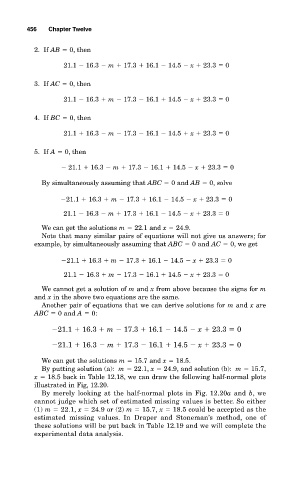
456   Chapter Twelve


             2. If AB   0, then
                     21.1   16.3   m   17.3   16.1   14.5   x   23.3   0

             3. If AC   0, then

                     21.1   16.3   m   17.3   16.1   14.5   x   23.3   0

             4. If BC   0, then

                     21.1   16.3   m   17.3   16.1   14.5   x   23.3   0

             5. If A   0, then
                       21.1   16.3   m   17.3   16.1   14.5   x   23.3   0

               By simultaneously assuming that ABC   0 and AB   0, solve

                      21.1   16.3   m   17.3   16.1   14.5   x   23.3   0
                     21.1   16.3   m   17.3   16.1   14.5   x   23.3   0

               We can get the solutions m   22.1 and x   24.9.
               Note that many similar pairs of equations will not give us answers; for
             example, by simultaneously assuming that ABC   0 and AC   0, we get

                      21.1   16.3   m   17.3   16.1   14.5   x   23.3   0

                     21.1   16.3   m   17.3   16.1   14.5   x   23.3   0
               We cannot get a solution of m and x from above because the signs for m
             and x in the above two equations are the same.
               Another pair of equations that we can derive solutions for m and x are
             ABC   0 and A   0:

                   21.1   16.3   m   17.3   16.1   14.5   x   23.3   0
                   21.1   16.3   m   17.3   16.1   14.5   x   23.3   0

               We can get the solutions m   15.7 and x   18.5.
               By putting solution (a): m   22.1, x   24.9, and solution (b): m   15.7,
             x   18.5 back in Table 12.18, we can draw the following half-normal plots
             illustrated in Fig, 12.20.
               By merely looking at the half-normal plots in Fig. 12.20a and  b,we
             cannot judge which set of estimated missing values is better. So either
             (1) m   22.1, x   24.9 or (2) m   15.7, x   18.5 could be accepted as the
             estimated missing values. In Draper and Stoneman’s method, one of
             these solutions will be put back in Table 12.19 and we will complete the
             experimental data analysis.

