Page 496 - Design for Six Sigma a Roadmap for Product Development

Fundamentals of Experimental Design 455

Half normal plot of the effects Half normal plot of the effects
(response is Y, Alpha = 0.05) (response is Y, Alpha = 0.05)
Effect type Effect type
98 Not significant 98 Not significant
Significant Significant
95 95
Factor Name Factor Name
A A A A
90 90
B B 85 B B
Percent 80 C C Percent 80 C C
85
70
60 70
60
50 50
40 40
30 30
20 20
10 10
0 0
0 1 2 3 4 5 6 7 0 1 2 3 4 5 6 7
Absolute effect Absolute effect
Lenth’s PSE = 2.175 Lenth’s PSE = 2.7
(a) ABC = 0, m = 24.7 (b) AB = 0, m = 19.5
Half normal plot of the effects Half normal plot of the effects
(response is Y, Alpha = 0.05) (response is Y, Alpha = 0.05)
Effect type Effect type
98 Not significant 98 Not significant
Significant Significant
95 Factor Name 95 Factor Name
A A A A
90 B C B C 90 B C B C
Percent 85 Percent 80
85
80
70 70
60 60
50 50
40 40
30 30
20 20
10 10
0 0
0 1 2 3 4 5 6 7 8 9 0 5 10 15 20
Absolute effect Absolute effect
Lenth’s PSE = 3.15 Lenth’s PSE = 7.8
(c) AC = 0, m = 18.3 (d) BC = 0, m = 40.3
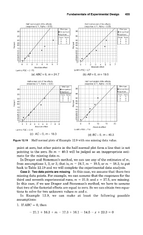
Figure 12.19 Half-normal plots of Example 12.9 with one missing data value.
point at zero, but other points in the half-normal plot form a line that is not
pointing to the zero. So m 40.3 will be judged as an inappropriate esti-
mate for the missing data m.
In Draper and Stoneman’s method, we can use any of the estimates of m,
from assumptions 1, 2, or 3, that is, m 24.7, m 19.5, or m 18.3, to put
back to Table 12.19 and we will complete the experimental data analysis.
Case 2: Two data points are missing In this case, we assume that there two
missing data points. For example, we can assume that the responses for the
third and seventh experimental runs, m 21.9, and x 27.5, are missing.
In this case, if we use Draper and Stoneman’s method, we have to assume
that two of the factorial effects are equal to zero. So we can obtain two equa-
tions to solve for two unknown values m and x.
In Example 12.9, we can make at least the following possible
assumptions:
1. If ABC 0, then
21.1 16.3 m 17.3 16.1 14.5 x 23.3 0