Page 501 - Design for Six Sigma a Roadmap for Product Development

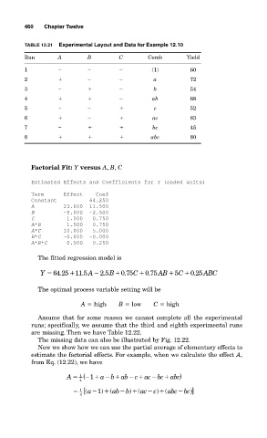
460 Chapter Twelve

TABLE 12.21 Experimental Layout and Data for Example 12.10
Run A B C Comb Yield
1 (1) 60
2 a 72
3 b 54
4 ab 68
5 c 52
6 ac 83
7 bc 45
8 abc 80

Factorial Fit: Y versus A, B, C

Estimated Effects and Coefficients for Y (coded units)
Term Effect Coef
Constant 64.250
A 23.000 11.500
B -5.000 -2.500
C 1.500 0.750
A*B 1.500 0.750
A*C 10.000 5.000
B*C -0.000 -0.000
A*B*C 0.500 0.250

The fitted regression model is

.
.
Y 64 25 11 5 A 2 5 B 0 75 C 0 75 AB 5 C 0 25 ABC
.
.
.
.
C
The optimal process variable setting will be
A high B low C high
Assume that for some reason we cannot complete all the experimental
runs; specifically, we assume that the third and eighth experimental runs
are missing. Then we have Table 12.22.
The missing data can also be illustrated by Fig. 12.22.
Now we show how we can use the partial average of elementary effects to
estimate the factorial effects. For example, when we calculate the effect A,
from Eq. (12.22), we have
1 (

A a babc ac bc abc)

1
4
[ ( a ( ab b)( ac abc bc)]
)(
c
1
1)
4