Page 504 - Design for Six Sigma a Roadmap for Product Development

Fundamentals of Experimental Design 463

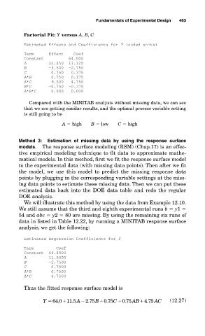
Factorial Fit: Y versus A, B, C
Estimated Effects and Coefficients for Y (coded units)
Term Effect Coef
Constant 64.000
A 22.250 11.125
B -5.500 -2.750
C 0.750 0.375
A*B 0.750 0.375
A*C 9.500 4.750
B*C -0.750 -0.375
A*B*C 0.000 0.000

Compared with the MINITAB analysis without missing data, we can see
that we are getting similar results, and the optimal process variable setting
is still going to be
A high B low C high

Method 3: Estimation of missing data by using the response surface
models. The response surface modeling (RSM) (Chap.17) is an effec-
tive empirical modeling technique to fit data to approximate mathe-
matical models. In this method, first we fit the response surface model
to the experimental data (with missing data points). Then after we fit
the model, we use this model to predict the missing response data
points by plugging in the corresponding variable settings at the miss-
ing data points to estimate these missing data. Then we can put these
estimated data back into the DOE data table and redo the regular
DOE analysis.
We will illustrate this method by using the data from Example 12.10.
We still assume that the third and eighth experimental runs b y1
54 and abc y2 80 are missing. By using the remaining six runs of
data in listed in Table 12.22, by running a MINITAB response surface
analysis, we get the following:

Estimated Regression Coefficients for Y
Term Coef
Constant 64.0000
A 11.5000
B -2.7500
C 0.7500
A*B 0.7500
A*C 4.7500

Thus the fitted response surface model is

.
.
.
.
Y 640 115 A 275 B 075 C 075 AB 475 AC (12.27)
.
.