Page 503 - Design for Six Sigma a Roadmap for Product Development

462 Chapter Twelve

Similarly,

⎤
c) ⎡
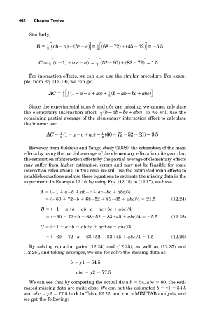
B 1 ⎡ ( ab a) ( bc ⎤ ⎦ 2 ⎣ ( 68 72) ( 45 52) 55

⎦
2 ⎣
1
.
a) ⎡
⎤
C 1 ⎡ ( c 1) ( ac ⎤ ⎦ 1 2 ⎣ ( 52 60) ( 83 72) 1..5
2 ⎣
⎦
For interaction effects, we can also use the similar procedure. For exam-
ple, from Eq. (12.19), we can get
AC ⎡ 1 2 1 ( a c ac ( b ab bc abc) ⎤ ⎦
)
2 ⎣

1
1
2
Since the experimental runs b and abc are missing, we cannot calculate

the elementary interaction effect 1 (bab bc abc ) , so we will use the
2
remaining partial average of the elementary interaction effect to calculate
the interaction:
AC 1 1 ( a c ac) 1 ( 60 72 52 83) 9 5
.
2 2
However, from Siddiqui and Yang’s study (2008), the estimation of the main
effects by using the partial average of the elementary effects is quite good, but
the estimation of interaction effects by the partial average of elementary effects
may suffer from higher estimation errors and may not be feasible for some
interaction calculations. In this case, we will use the estimated main effects to
establish equations and use those equations to estimate the missing data in the
experiment. In Example 12.10, by using Eqs. (12.15) to (12.17), we have
A ( 1 a b ab c ac bc abc)/4
( 60 72 b 68 52 83 45 abc)/4 21.5 (12.24)
B ( 1 a b ab c ac bc abc)/4
( 60 72 b 68 52 83 45 abc)/4 5.5 (12.25)
C ( 1 a b ab c ac bc abc)/4
( 60 72 b 68 52 83 45 abc)/4 1.5 (12.26)

By solving equation pairs (12.24) and (12.25), as well as (12.25) and
(12.26), and taking averages, we can for solve the missing data as

b y1 54.5
abc y2 77.5
We can see that by comparing the actual data b 54, abc 80, the esti-
mated missing data are quite close. We can put the estimated b y1 54.5
and abc y2 77.5 back in Table 12.22, and run a MINITAB analysis, and
we get the following: