Page 495 - Design for Six Sigma a Roadmap for Product Development

454 Chapter Twelve

effects. In this case, Draper and Stoneman’s method is able to select a “best
assumption” (regarding which factorial effect to be assumed zero), with the
aid of a half-normal plot.
Specifically, in Example 12.9 suppose we can make one of the following
assumptions:
1. If ABC 0, then we can solve for m 24.7.
2. If AB 0, then we have
21.1 16.3 m 17.3 16.1 14.5 27.5 23.3 0

and this leads to m 19.5.
3. If AC 0, then we have
21.1 16.3 m 17.3 16.1 14.5 27.5 23.3 0

and this leads to m 18.3.
4. If BC 0, then we have
21.1 16.3 m 17.3 16.1 14.5 27.5 23.3 0

and this leads to m 40.3.
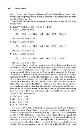
So the question is, which m should we use, if we don’t know the actual
value of m? Draper and Stoneman proposed to put all these m values back
into the experimental data table one at a time, and then we can plot the esti-
mated factorial effects into the half-normal plot, proposed by Cuthbert
Daniel (1976). In Daniel’s point of view, when we put a good set of factorial
experimental data into the half-normal plot, there are some nonsignificant
effects; these nonsignificant effects should form a scatter of dots pointing to
the origin of the zero point in the half-normal plot, and the significant
effects are outliers. If we find that the scatter of low effects points does not
point to the zero point, then this data set does not behave normally and it
could be a data set with wrong values. For Example 12.9 with one missing
data value, we plotted four half-normal plots in Fig.12.19, with the afore-
mentioned four assumptions:
1. ABC 0, m 24.7
2. AB 0, m 19.5
3. AC 0, m 18.3
4. BC 0, m 40.3
We can see from Fig. 12.19 that for assumptions 1, 2, and 3 there is
always one point whose effect is zero; this point corresponds to the point
related to the assumption. For example, in Fig. 12.19a, this point corresponds
to ABC 0. Also there are several other points whose effects are small, and
they form a line segment that points to zero. So the estimated missing val-
ues (m 24.7, m 19.5, m 18.3), corresponding to assumptions 1, 2, and 3
are acceptable estimated values, according to Draper and Stoneman’s
method. But for assumption 4, we can see that in Fig. 12.19d there is one