Page 300 - Distributed model predictive control for plant-wide systems

274 Distributed Model Predictive Control for Plant-Wide Systems

80

70

60

Velocity (m/s) 50

40

30

20

10
4
3
2

1 40 50 60
Coach numbers 0 10 20 30
Simulation steps

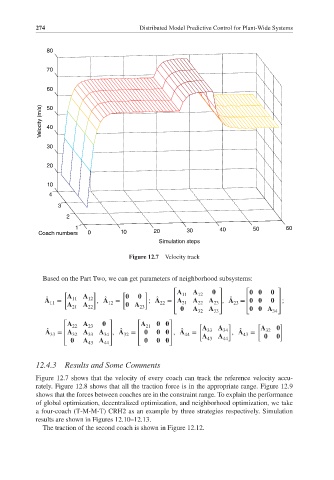
Figure 12.7 Velocity track

Based on the Part Two, we can get parameters of neighborhood subsystems:
[ ] [ ] ⎡A 11 A 12 ⎤ ⎡ ⎤
A 11 A 12
̂
̂
̂
̂
A 11 = , A 12 = ; A 22 = A 21 A 22 A 23 ⎥ , A = ⎥ ;
⎢
⎢
23
A
21 A 22 A 23 ⎣ A 32 A ⎦ ⎥ ⎢ 34 ⎥
⎢
33
⎣ A ⎦
⎡A A ⎡A [ ] [ ]
22 23 ⎤ 21 ⎤ A A A
̂
̂
̂
̂
A = A A A ⎥ , A = ⎢ , A = 33 34 , A = 32
⎢
⎥
33 32 33 34 32 44 A A 43
⎣ A 43 A ⎦ ⎥ ⎣ ⎦ ⎥ 43 44
⎢
⎢
44
12.4.3 Results and Some Comments
Figure 12.7 shows that the velocity of every coach can track the reference velocity accu-
rately. Figure 12.8 shows that all the traction force is in the appropriate range. Figure 12.9
shows that the forces between coaches are in the constraint range. To explain the performance
of global optimization, decentralized optimization, and neighborhood optimization, we take
a four-coach (T-M-M-T) CRH2 as an example by three strategies respectively. Simulation
results are shown in Figures 12.10–12.13.
The traction of the second coach is shown in Figure 12.12.