Page 297 - Distributed model predictive control for plant-wide systems

High-Speed Train Control with Distributed Predictive Control 271

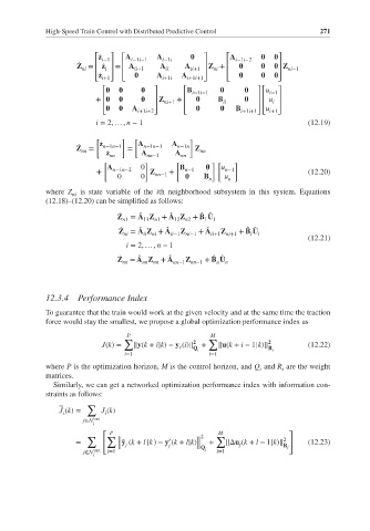
⎡ ̇ z i−1 ⎤ ⎡A i−1i−1 A i−1i ⎤ ⎡A i−1i−2 ⎤
Z = ⎢ ̇ z ⎥ = ⎢ A A A ⎥ Z + ⎢ Z
̇
⎥
ni i ii−1 ii ii+1 ni ni−1
⎢ ⎥ ⎢ ⎥ ⎢ ⎥
⎣ ̇ z i+1⎦ ⎣ A i+1i A i+1i+1⎦ ⎣ ⎦
⎡ ⎤ ⎡B i−1i−1 ⎤ ⎡u i−1 ⎤
+ ⎥ Z ni+1 + ⎢ B ii ⎥ ⎢ u i ⎥
⎢
⎣ A i+1i+2⎦ ⎥ ⎢ B i+1i+1⎦ ⎣ u i+1⎦ ⎥
⎢
⎥ ⎢
⎣
i = 2, … , n − 1 (12.19)
[ ] [ ]
Z = ̇ z n−1n−1 = A n−1n−1 A n−1n Z
̇
nn ̇ z nn A nn−1 A nn nn
[ ] [ ][ ]
+ A n−1n−2 0 Z + B n−1 u n−1 (12.20)
0 0 nn−1 B u
n n
where Z is state variable of the ith neighborhood subsystem in this system. Equations
ni
(12.18)–(12.20) can be simplified as follows:
̂
̂
̂ ̂
Z ̇ = A Z + A Z + B U
n1 11 n1 12 n2 1 1
̂
̇
Z
Z
̂ ̂
̂
Z = A Z + A ii−1 ni−1 + A ii+1 ni+1 + B U i
̂
ni
ii ni
i
(12.21)
i = 2, … , n − 1
̂
̂
̇
Z
̂ ̂
Z = A Z + A nn−1 nn−1 + B U n
nn
n
nn nn
12.3.4 Performance Index
To guarantee that the train would work at the given velocity and at the same time the traction
force would stay the smallest, we propose a global optimization performance index as
P M
∑ ∑
J(k)= + (12.22)
r Q i ‖u(k + i − 1|k)‖ R i
‖y(k + i|k)− y (i)‖
i=1 i=1
where P is the optimization horizon, M is the control horizon, and Q and R are the weight
i
i
matrices.
Similarly, we can get a networked optimization performance index with information con-
straints as follows:
∑
J (k)= J (k)
i
i
out
j∈N
i
[ ]
P M
∑ ∑ r 2 ∑ 2
= ‖ j j ‖ + ‖Δu (k + l − 1|k)‖ (12.23)
‖̂ y (k + l |k) − y (k + l|k)‖
j
‖ ‖Q j R j
out l=1 l=1
j∈N
i