Page 296 - Distributed model predictive control for plant-wide systems

270 Distributed Model Predictive Control for Plant-Wide Systems

V

Predictor1 MPC2 MPC3 MPCi Predictor1

u 1 u 2 u 3 u i u n
x 1
x 2 x i–1 x i
1 2 3 i n
W 02
W 03 W 0i W 0n
W 01
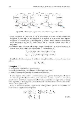
Figure 12.5 The structure diagram of the distributed model predictive control

Adjacent subsystems. If subsystems S and S interact with each other and the output of the
i
j
subsystem S is the input of the subsystem S , subsystem S is called the input-adjacent
i
j
j
subsystem of the subsystem S and subsystem S is called the output-adjacent subsystem
i
i
of the subsystem S . By this way, subsystems S and S are called adjacent subsystems or
j
i
j
neighbors.
Neighborhood of the subsystem. All the input (output) of neighbor’s set of the subsystem S is
i
defined as the input (output) of neighborhood P of subsystem S :
+i i
P +i ={S , S |S is the input neighbor of S }
i
j
j
i
P ={S , S |S is the output neighbor of S }
−i i j j i
Neighborhood of the subsystem S : all the set of neighbors of the subsystem S is shown as
i i
follows:
P = P ∪ P −i
i
+i
Assumption 12.1
(a) subsystems’ controllers act synchronously;
(b) during a sample time, the controllers contact others only once;
(c) there is one step delay during the communication course.
It is not rigorous for these three assumptions in the real systems. Normally the calculation
time is much longer than the sample time, so the assumption (a) is not rigorous. The assumption
(b) is to reduce the network communication between the controllers and improve the reliability
of the algorithm. In the real systems, the instantaneous communication is not existence, so the
assumption (c) is necessary.
Based on the definition of the neighborhood, the longitudinal dynamic model (12.17) can
be rewritten as neighborhood subsystems
[ ] [ ] [ ]
Z = ̇ z 1 = A 11 A 12 Z + Z n2
̇
n1
n1
̇ z
2 A 21 A 22 A 23
[ ][ ]
+ B 1 u 1 (12.18)
B 2 u 2