Page 541 - Dynamics of Mechanical Systems

0593_C15_fm Page 522 Tuesday, May 7, 2002 7:05 AM

522 Dynamics of Mechanical Systems

Next, consider the addition of a particle P with mass m and coordinates (x, y) as in
Figure 15.5.1. The components of the inertia dyadic of P relative to A relative to n , n ,
y
x
and n are (see Eq. (7.3.11)):
z
 y 2 − xy 0 

I = m − xy x 2 0  (15.5.10)
P
ij  
2
2
 0 0 x + y  

Suppose P is attached to one of the rods. Then, by inspection of Eqs. (15.5.3) to (15.5.6),
we see that, with the zeroes in the third rows and columns of the inertia matrix of Eq.
(15.5.10) and with both ωω ωω and ωω ωω having only components along n , there is no contri-
BC
z
AB
bution to the inertia torques with components along n or n . This means that for the
x
y
purposes of balancing we can focus our attention upon reducing the magnitudes of the
inertia forces in the X–Y plane.
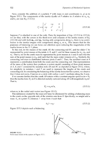
To this end, let the masses of the crank AB, the connecting rod BC, and the slider C be
represented by point masses at the joints A, B, and C, and let these masses be m , m , and
B
A
m . That is, we let the crank mass be represented by point masses at A and B such that the
C
sum of the point masses is m and such that the mass center remains at G . Similarly, the
AB
AB
connecting rod mass is distributed between joints B and C. Then, the resultant mass at B
represents a contribution from both the crank and the connecting rod. This representation
of the mass of the system then produces a system model consisting of three point masses
at A, B, and C connected by massless rods AB and BC as depicted in Figure 15.5.2, where,
for simplicity in notation, r and are used to represent the lengths of the crank and
connecting rod. In considering the balancing of the inertia forces for this system, we observe
that A does not move, B moves on a circle with radius r, and C oscillates along the X-axis.
˙
θ
If we assume further that the crank AB rotates with a constant angular speed ω (ω = ),
then the inertia force F * on B is directed radially outward along AB with magnitude m rω .
2
B B
That is,
F = mrω 2 n (15.5.11)
*
B B r
where n is the radial unit vector (see Figure 15.5.2).
r
This imbalance created by the mass at B may be eliminated by adding a balancing mass
to the crank on the opposite side of the rotation axis from B. Specifically, we might add a
ˆ
mass ˆ m at a point a distance away from A such that:
B
ˆ r
B
ˆˆ =
mr mr (15.5.12)
B B
Figure 15.5.3 depicts such a balancing.
Y
n r
B(m )
B
r

θ φ C(m )
FIGURE 15.5.2 C
A(m ) X
A
Point mass model of the system of Figure 15.5.1.