Page 542 - Dynamics of Mechanical Systems

0593_C15_fm Page 523 Tuesday, May 7, 2002 7:05 AM

Balancing 523

Y
B

r
y

A θ φ C(m )
C
x X

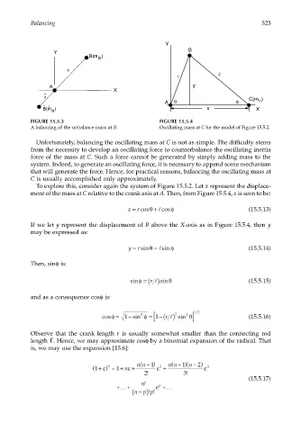
FIGURE 15.5.3 FIGURE 15.5.4
A balancing of the unbalance mass at B. Oscillating mass at C for the model of Figure 15.5.2.

Unfortunately, balancing the oscillating mass at C is not as simple. The difficulty stems
from the necessity to develop an oscillating force to counterbalance the oscillating inertia
force of the mass at C. Such a force cannot be generated by simply adding mass to the
system. Indeed, to generate an oscillating force, it is necessary to append some mechanism
that will generate the force. Hence, for practical reasons, balancing the oscillating mass at
C is usually accomplished only approximately.
To explore this, consider again the system of Figure 15.5.2. Let x represent the displace-
ment of the mass at C relative to the crank axis at A. Then, from Figure 15.5.4, x is seen to be:

x = cosθ + cosφ (15.5.13)
l
r
If we let y represent the displacement of B above the X-axis as in Figure 15.5.4, then y
may be expressed as:

y = sinθ = sinφ (15.5.14)
l
r
Then, sinφ is:

r
sinφ = ( ) l sinθ (15.5.15)

and as a consequence cosφ is:

2
2
r
cosφ = 1 − sin φ =[ 1 −( ) l 2 sin θ] / 12 (15.5.16)
Observe that the crank length r is usually somewhat smaller than the connecting rod
length . Hence, we may approximate cosφ by a binomial expansion of the radical. That
is, we may use the expansion [15.6]:

( 1+ ) =+ ε n + ( nn − 1) ε 2 + ( nn − 1)(n − 2) ε 3
n
ε
1
2! 3!
(15.5.17)
+…+ n! ε p +…
− ) p!!
(np