Page 331 - Electrical Properties of Materials

Semiconductor lasers 313
2
number of possible states are πn , since there is a state for each integer value
2
2
2
of n y and n z . Solving for n = n + n from eqn (12.41) we obtain
z
y
2
E
l
2
n π = π –1 . (12.43)
d E 0
∗
Thus, eqn (12.43) gives the number of states having energies less than E. ∗ This is exactly analogous to the calcu-
Similarly, the number of states having energies less than E +dE is lation of the three-dimensional density
of states we performed in Section 6.2.
2

l E + dE
π –1 . (12.44)
d E 0
Consequently, the states having energies between E and E +dE (and that
defines the density of states function Z(E)) may be found as
l dE
2
Z(E)dE = π . (12.45)
d E 0
Remember that only positive integers count, so we need to divide by 4. On
the other hand, there is spin as well, which is taken into account by multiplying
by 2. Thus, the density of states in eqn (12.45) needs to be divided by 2. That
is actually a minor detail. The important thing is that the density of states is
independent of energy in the range n x =1 to n x = 2. Taking l = 300 μm and
8
8
2
2
2
2
d = 10 nm, we get (l/d) =9×10 . Thus, when n = n +n =27×10 , then E Two-dimensional
z
y
density of states
reaches the value of 4E 0 . We may alternatively, however, obtain an energy 4E 0
with n y and n z being very small and n x = 2. It is clear that above 4E 0 ,the same
energy level may be reached in two different ways: with n y and n z relatively
small and n x = 2, or with n y and n z large and n x = 1. Thus, the number of
available states suddenly doubles at E =4E 0 . Between E =4E 0 and E =9E 0 ,
the density of states remains constant again, and there is a new contribution at
E =9E 0 , which leads to trebling of the initial density of states.
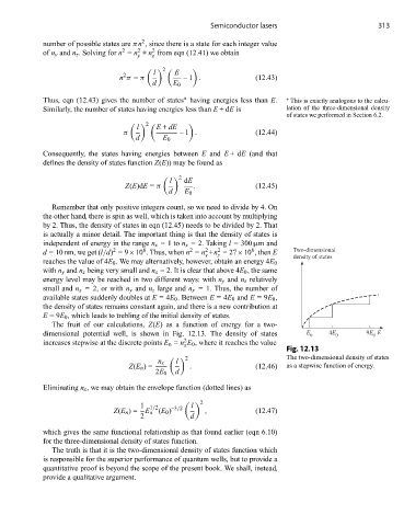
The fruit of our calculations, Z(E) as a function of energy for a two-
dimensional potential well, is shown in Fig. 12.13. The density of states E 0 4E 0 9E E
0
2
increases stepwise at the discrete points E n = n E 0 , where it reaches the value
x
Fig. 12.13
2 The two-dimensional density of states
n x l
Z(E n )= . (12.46) as a stepwise function of energy.
2E 0 d
Eliminating n x , we may obtain the envelope function (dotted lines) as
2
1 1/2 –3/2 l

Z(E n )= E n (E 0 ) , (12.47)
2 d
which gives the same functional relationship as that found earlier (eqn 6.10)
for the three-dimensional density of states function.
The truth is that it is the two-dimensional density of states function which
is responsible for the superior performance of quantum wells, but to provide a
quantitative proof is beyond the scope of the present book. We shall, instead,
provide a qualitative argument.