Page 302 - Elements of Distribution Theory

P1: JZP
052184472Xc09 CUNY148/Severini June 2, 2005 12:8

288 Approximation of Integrals

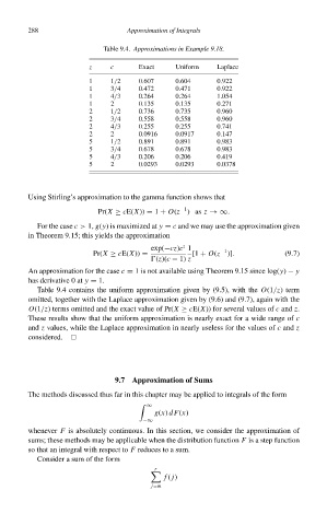
Table 9.4. Approximations in Example 9.18.

z c Exact Uniform Laplace

1 1/2 0.607 0.604 0.922
1 3/4 0.472 0.471 0.922
1 4/3 0.264 0.264 1.054
1 2 0.135 0.135 0.271
2 1/2 0.736 0.735 0.960
2 3/4 0.558 0.558 0.960
2 4/3 0.255 0.255 0.741
2 2 0.0916 0.0917 0.147
5 1/2 0.891 0.891 0.983
5 3/4 0.678 0.678 0.983
5 4/3 0.206 0.206 0.419
5 2 0.0293 0.0293 0.0378

Using Stirling’s approximation to the gamma function shows that
−1
Pr(X ≥ cE(X)) = 1 + O(z )as z →∞.
For the case c > 1, g(y)is maximized at y = c and we may use the approximation given
in Theorem 9.15; this yields the approximation
z
exp(−cz)c 1 −1
Pr(X ≥ cE(X)) = [1 + O(z )]. (9.7)
(z)(c − 1) z
An approximation for the case c = 1is not available using Theorem 9.15 since log(y) − y
has derivative 0 at y = 1.
Table 9.4 contains the uniform approximation given by (9.5), with the O(1/z) term
omitted, together with the Laplace approximation given by (9.6) and (9.7), again with the
O(1/z) terms omitted and the exact value of Pr(X ≥ cE(X)) for several values of c and z.
These results show that the uniform approximation is nearly exact for a wide range of c
and z values, while the Laplace approximation in nearly useless for the values of c and z
considered.

9.7 Approximation of Sums
The methods discussed thus far in this chapter may be applied to integrals of the form
∞

g(x) dF(x)
−∞
whenever F is absolutely continuous. In this section, we consider the approximation of
sums; these methods may be applicable when the distribution function F is a step function
so that an integral with respect to F reduces to a sum.
Consider a sum of the form
r

f ( j)
j=m