Page 440 - Engineering Digital Design

410 CHAPTER 9 / PROPAGATION DELAY AND TIMING DEFECTS

Static 1 Static 0
Hazards Hazards
A\ 1
A[1,2] BXYZ < > BXYZ
N A Jl I A |0
__ r
A[2,3] BYZ

_ - J A }1 f A 10
A[1,3] BXYZ < > BXYZ
A/ 1
8
, , - f' ! 0
B[1,2] AXYZ < > AXYZ
^ B/1 [ B |0
(b)
Dynamic Hazards
/A\ 0 / A\ 1
A[1,2,3] BXYZ < > BXYZ < >
\A/1 \A/0
(C)
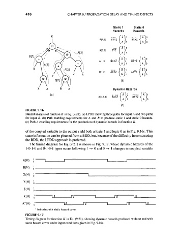
FIGURE 9.16
Hazard analysis of function K in Eq. (9.21). (a) LPDD showing three paths for input A and two paths
for input B. (b) Path enabling requirements for A and B to produce static 1 and static 0 hazards,
(c) Path A enabling requirements for the production of dynamic hazards in function K.

of the coupled variable to the output yield both a logic 1 and logic 0 as in Fig. 9.16c. This
same information can be gleaned from a BDD, but, because of the difficulty in constructing
the BDD, the LPDD approach is preferred.
The timing diagram for Eq. (9.21) is shown in Fig. 9.17, where dynamic hazards of the
1-0-1-0 and 0-1-0-1 types occur following 1 —> 0 and 0 -> 1 changes in coupled variable

K(H) J - LJI _ TU - 1 _ (1 - Ul

K*(H) J - Ul _ n - 1 _ (1
* Indicates with static hazard cover
FIGURE 9.17
Timing diagram for function K in Eq. (9.21), showing dynamic hazards produced without and with
static hazard cover under input conditions given in Fig. 9.16c.