Page 94 - Enhancing CAD Drawings with Photoshop

4386.book Page 77 Monday, November 15, 2004 3:27 PM
WORKING WITH DIGITAL FILM 77

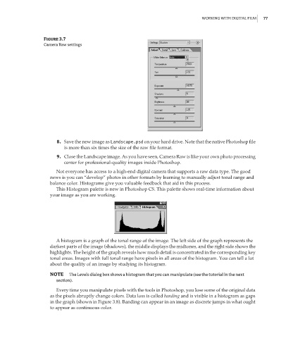
Figure 3.7
Camera Raw settings

8. Save the new image as Landscape.psd on your hard drive. Note that the native Photoshop file
is more than six times the size of the raw file format.
9. Close the Landscape image. As you have seen, Camera Raw is like your own photo processing
center for professional-quality images inside Photoshop.

Not everyone has access to a high-end digital camera that supports a raw data type. The good
news is you can “develop” photos in other formats by learning to manually adjust tonal range and
balance color. Histograms give you valuable feedback that aid in this process.
This Histogram palette is new in Photoshop CS. This palette shows real-time information about
your image as you are working.

A histogram is a graph of the tonal range of the image. The left side of the graph represents the
darkest parts of the image (shadows), the middle displays the midtones, and the right side shows the
highlights. The height of the graph reveals how much detail is concentrated in the corresponding key
tonal areas. Images with full tonal range have pixels in all areas of the histogram. You can tell a lot
about the quality of an image by studying its histogram.
NOTE The Levels dialog box shows a histogram that you can manipulate (see the tutorial in the next
section).
Every time you manipulate pixels with the tools in Photoshop, you lose some of the original data
as the pixels abruptly change colors. Data loss is called banding and is visible in a histogram as gaps
in the graph (shown in Figure 3.8). Banding can appear in an image as discrete jumps in what ought
to appear as continuous color.