Page 135 - Excel Timesaving Techniques for Dummies

25_574272 ch22.qxd 10/1/04 10:45 PM Page 120
120
Technique 22: Charting Data in a Snap
studied, step-by-step way to generate your charts 2. Select the general type of chart in the Chart
via its Chart Wizard. Type list box, select the specific type in the
Chart Sub-type palette, and then click the Next
Although creating a new chart with the Chart Wizard button.
is a little slower process, it’s also one that gives you
the opportunity to make basic enhancements — To get an idea of how your data will look dressed
selecting a new chart type, adding chart titles, and up in the selected chart type, click and hold down
so on — as you create the chart. So, when you’re the Press and Hold Down to View Sample button.
finished, you have a chart that requires much less When you click the Next button, Excel opens the
futzing on your part. When looked at from this per- Step 2 of 4 - Chart Source Data dialog box, shown
spective, you may find that the Chart Wizard, while in Figure 22-7.
not nearly as flashy, may actually prove to be more
efficient.
To graph your data with the Chart Wizard, follow
these general steps:

1. Select the data in the spreadsheet that you
want represented in the chart and then click
the Chart Wizard button (the one sporting the
column chart icon) on the Standard toolbar or
choose Insert➪Chart.
Excel opens the Step 1 of 4 - Chart Type dialog
box, shown in Figure 22-6.

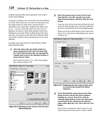
• Figure 22-7: Designating the data range and data series
to be used in the second Chart Wizard
dialog box.

3. Check that both the range shown in the Data
Range text box and the selected worksheet
charting are correct. If need be, click the
Columns option button to have the data series
represented by the columns in the selected
range rather than the rows. Then click the Next
button.
• Figure 22-6: Selecting the type of chart in the first Chart
Wizard dialog box. If you need to change the values used for a par-
ticular data point in the series or add or delete